Centrifugal impeller CFX tutorial

Centrifugal impeller CFX tutorial#

This tutorial shows how to use the barotropy Python package to generate barotropic property models and use them in ANSYS CFX.

You can download the CFX files used in this tutorial from this GitHub release.

1. Installation#

Create a clean Python environment and install barotropy.

Option 1: Using Conda#

If you use miniconda to manage your virtual environemnts

conda create -n barotropy-env python=3.10 -y
conda activate barotropy-env
pip install barotropy

Option 2: Using Python `venv`#

If you prefer to avoid conda you can also create a lightweight virtual environmnet using venv. If you are using git-bash on windows

python -m venv env
source env/Scripts/activate
python -m pip install barotropy

Or if you are using Linux or mcOS

python3 -m venv env
source env/bin/activate
pip install barotropy

2. Generate the barotropic model#

To generate the barotropic model, simply run the script:

python create_barotropic_model.py

This will:

Simulate a barotropic expansion of CO₂
Fit polynomial expressions for key properties
Export CFX-compatible expressions in barotropic_model/CFX_expressions.txt
Save plots and polynomial data in the barotropic_model/ folder

Below is a breakdown of the main script components.

Step 2.1: Define the fluid and thermodynamic conditions#

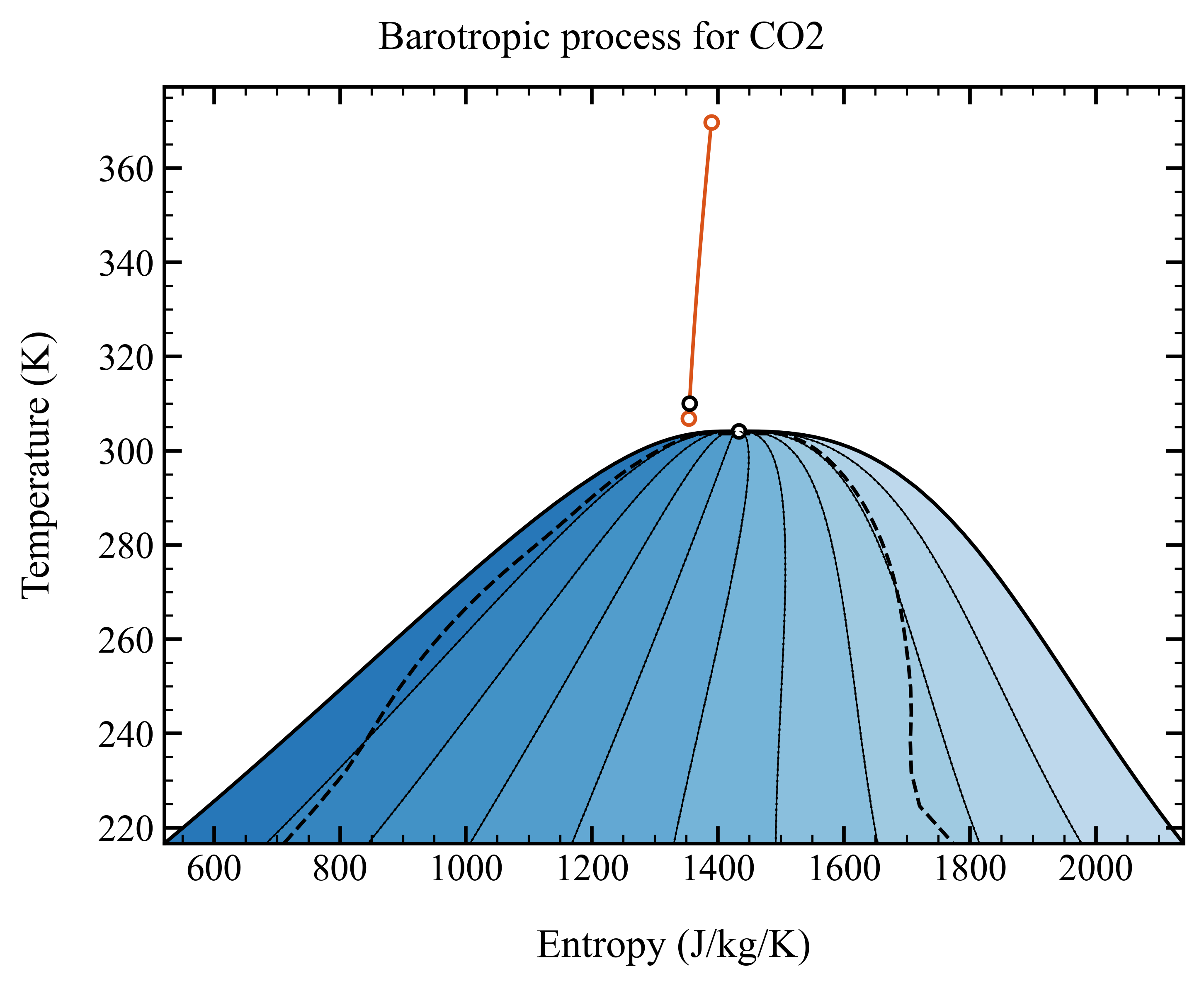
We use CO₂, compressing from 310 K and 90 bar. The maximum (outlet) pressure is set to five times the inlet pressure to cover a broad range of thermodynamic states. The minimum pressure is set to 90 % of the inlet pressure to ensure that properties at slightly lower pressures are available—relevant for modeling fluid acceleration at the impeller inlet.

fluid_name = "CO2"
fluid = bpy.Fluid(name=fluid_name, backend="HEOS")
T_in = 310.0       # [K]
p_in = 90.0e5      # [Pa]
p_min = 5.0*p_in   # [Pa]
p_max = 0.9*p_in   # [Pa]

The corresponding expansion is illustrated in the temperature-entropy diagram below

Step 2.2: Set up the barotropic model#

We assume thermodynamic equilibrium during compression, which is not an issue for single-phase flow, and specify a polytropic efficiency of 80 %. The barotropic model is set up to fit fifth-degree polynomials for the variables listed in polynomial_variables. Since both p_min and p_max are provided, we must explicitly specify process_type="compression", as the direction of the process cannot be inferred from the inlet and outlet pressures.

model = bpy.BarotropicModel(
    fluid_name=fluid_name,
    T_in=T_in,
    p_in=p_in,
    p_min=p_min,
    p_max=p_max,
    efficiency=0.8,
    process_type="compression",
    calculation_type="equilibrium",
    HEOS_solver="hybr",
    ODE_solver="LSODA",
    ODE_tolerance=1e-9,
    polynomial_degree=5,
    polynomial_format="horner",
    output_dir=DIR_OUT,
    polynomial_variables=["density", "viscosity", "speed_sound", "void_fraction", "vapor_quality"],
)

Step 2.3: Solve, export, and visualize#

We evaluate the expansion, fit the polynomials, export the expressions, and generate plots of the thermodynamic path and fitting error for each variable.

model.solve()
model.fit_polynomials()
model.export_expressions_fluent(output_dir=DIR_OUT)
model.export_expressions_cfx(output_dir=DIR_OUT)

model.poly_fitter.plot_phase_diagram(
    fluid=fluid,
    var_x="s",
    var_y="T",
    savefig=True,
    showfig=True,
    plot_spinodal_line=True,
)

for var in model.poly_fitter.variables:
    model.poly_fitter.plot_polynomial_and_error(
        var=var,
        savefig=True,
        showfig=True,
    )

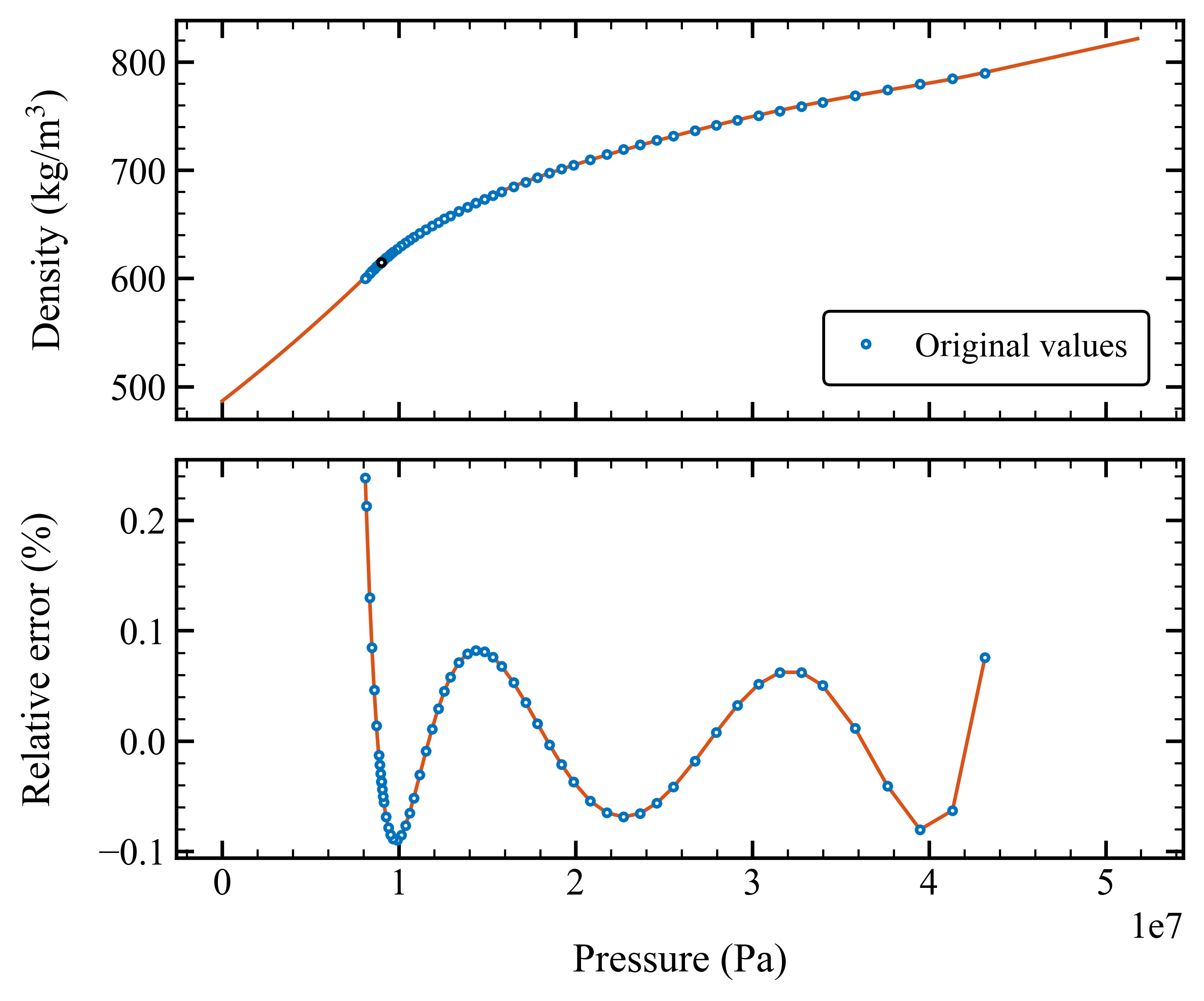
The barotropic model for density is shown below. For pressures below p_min, an exponential extrapolation ensures that the density remains positive and decreases monotonically. This safeguard is important during internal CFD iterations, where unphysical negative pressures may temporarily arise and require physically plausible density values to support convergence.

3. Use the barotropic model in CFX#

This case is based on a centrifugal compressor impeller. The geometry provided should work out of the box, but you can modify it if needed.

To adjust the geometry or mesh:

Open the centrifugal_impeller.wbpj Workbench file.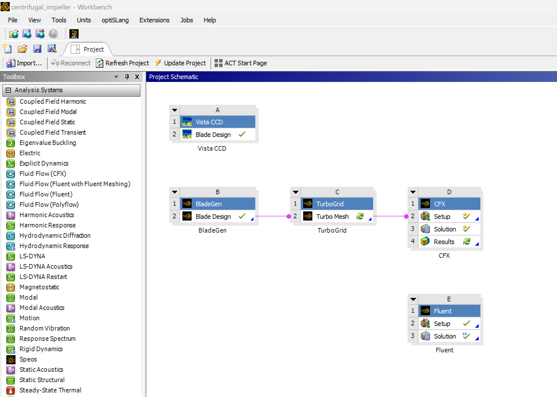
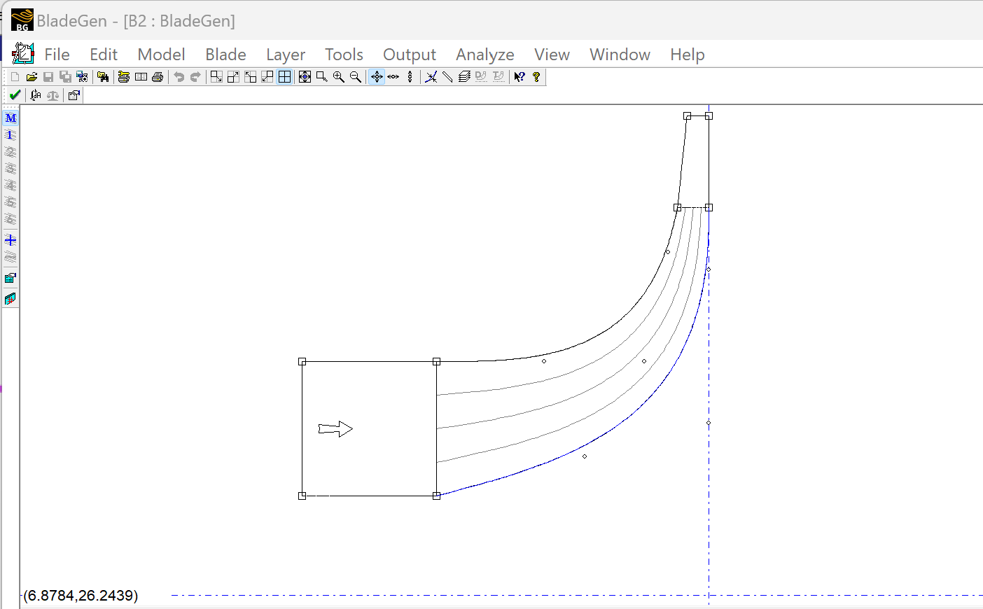
Use Ansys BladeGen to modify the impeller geometry:
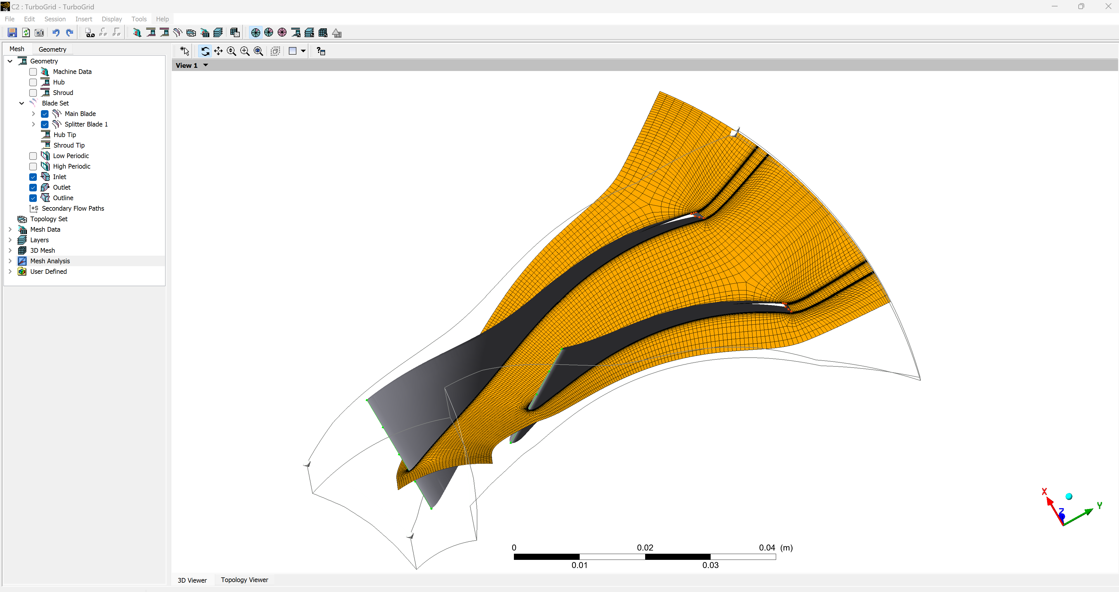
Adjust the mesh settings in Ansys TurboGrid:

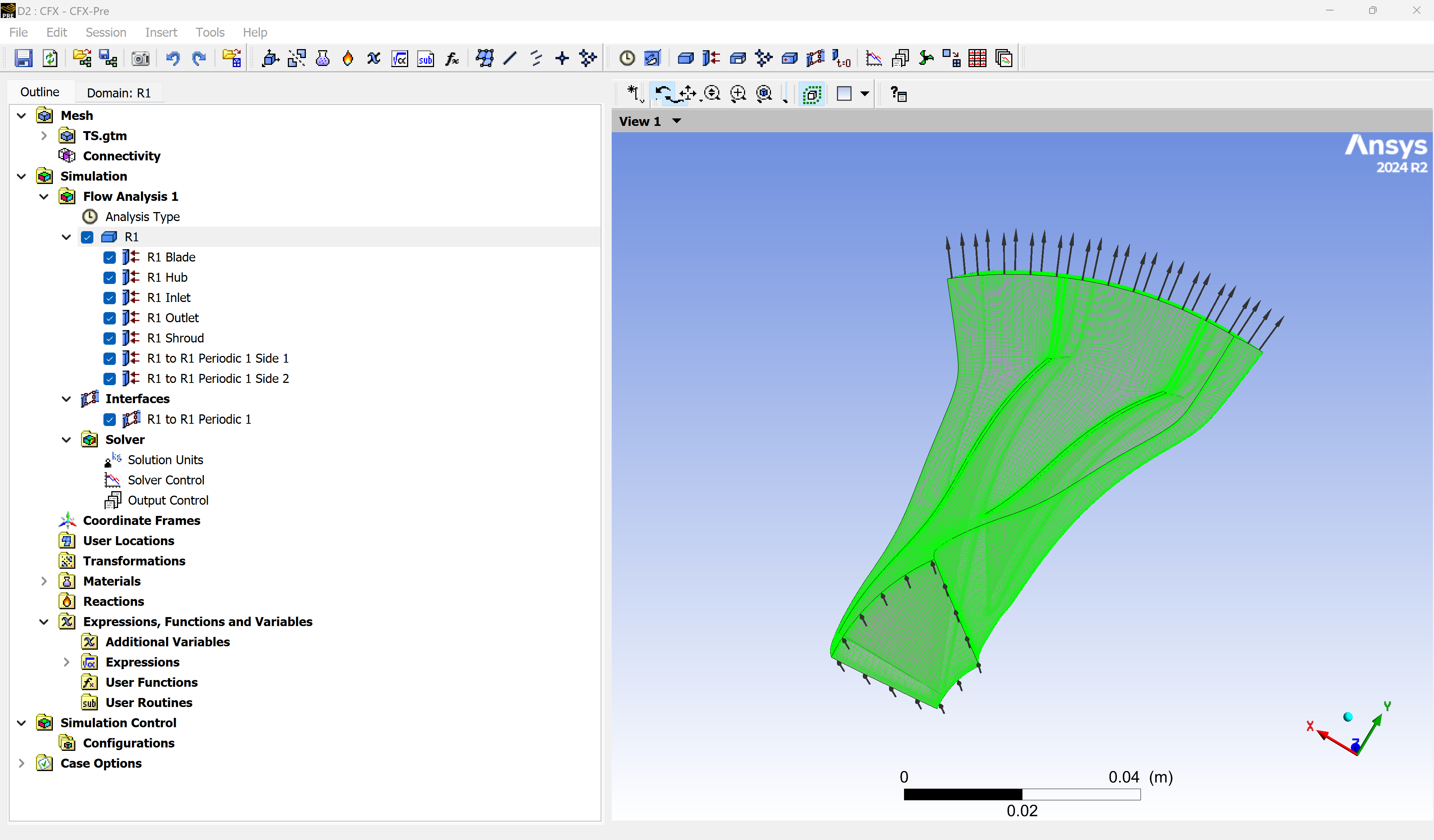
Once the mesh is ready, open Ansys CFX-Pre to configure the CFD simulation:

CFX-Pre

Step 3.2: Check CFX expressions#

Open the file barotropic_model/cfx_expressions.txt. It contains CFX-compatible expressions for:

barotropic_density
barotropic_viscosity
barotropic_speed_sound
barotropic_void_fraction
barotropic_vapor_quality

Each expression is defined as a function of absolute pressure in Pascal. Example snippet:

CFX expressions for barotropic properties
Creation datetime: 2025-04-01 21:46:00.584473

barotropic_density
(if(Absolute Pressure >= 4.3172602232385412e+07 [Pa],
7.9029740467060265e+02 + 1.5585573580243636e+02 * (Absolute Pressure / 4.3172602232385412e+07 [Pa] - 1.0000000000000000e+00),
if(Absolute Pressure >= 8.1000000000000075e+06 [Pa],
3.7719286741630594e+02 + (Absolute Pressure / 4.3172602232385412e+07 [Pa]) *
(1.9069634173268196e+03 + (Absolute Pressure / 4.3172602232385412e+07 [Pa]) *
(-5.0217902319823761e+03 + (Absolute Pressure / 4.3172602232385412e+07 [Pa]) *
(7.5391828666755409e+03 + (Absolute Pressure / 4.3172602232385412e+07 [Pa]) *
(-5.7311817562421811e+03 + (Absolute Pressure / 4.3172602232385412e+07 [Pa]) *
(1.7199302414764936e+03))))),
6.0129371881930194e+02 * exp((Absolute Pressure / 4.3172602232385412e+07 [Pa] - 0.1876189893859094) / (8.8685400882947685e-01))))) * 1 [kg/m^3]

barotropic_viscosity
(if(Absolute Pressure >= 4.3172602232385412e+07 [Pa],
7.2125104547306039e-05 + 2.5165884862101540e-05 * (Absolute Pressure / 4.3172602232385412e+07 [Pa] - 1.0000000000000000e+00),
if(Absolute Pressure >= 8.1000000000000075e+06 [Pa],
2.0001983602077405e-05 + (Absolute Pressure / 4.3172602232385412e+07 [Pa]) *
(1.9944217404247922e-04 + (Absolute Pressure / 4.3172602232385412e+07 [Pa]) *
(-4.8758152175582535e-04 + (Absolute Pressure / 4.3172602232385412e+07 [Pa]) *
(7.2428379252763341e-04 + (Absolute Pressure / 4.3172602232385412e+07 [Pa]) *
(-5.4814199609366592e-04 + (Absolute Pressure / 4.3172602232385412e+07 [Pa]) *
(1.6412067222460730e-04))))),
4.4400199113488022e-05 * exp((Absolute Pressure / 4.3172602232385412e+07 [Pa] - 0.1876189893859094) / (5.5845319585495468e-01))))) * 1 [Pa*s]

Step 3.3: Define custom named expressions#

Navigate to “Expressions, Functions and Variables” in the Outline, then open the Expressions Editor.

Create two expressions:

barotropicDensity
barotropicViscosity

Copy and paste the corresponding content from barotropic_model/cfx_expressions.txt into each expression field.

You can plot the expressions directly in CFX to verify correctness. Note that CFX-Pre uses single-precision arithmetic, so high-degree or ill-conditioned polynomials may not display correctly. Using polynomial degrees between 4 and 6 typically gives good results.

CFX-Pre-expressions

Step 3.4: Create a barotropic fluid and assign expressions#

Define a new fluid in CFX:

Set Density and Dynamic Viscosity as Expressions, using the previously defined functions (e.g., barotropicDensity, barotropicViscosity)
Specify a dummy value for heat capacity (this is required by CFX even if not used)
Set minimum and maximum limits for Absolute Pressure. It’s not clear how CFX handles these limits internally

CFX-Pre-fluid

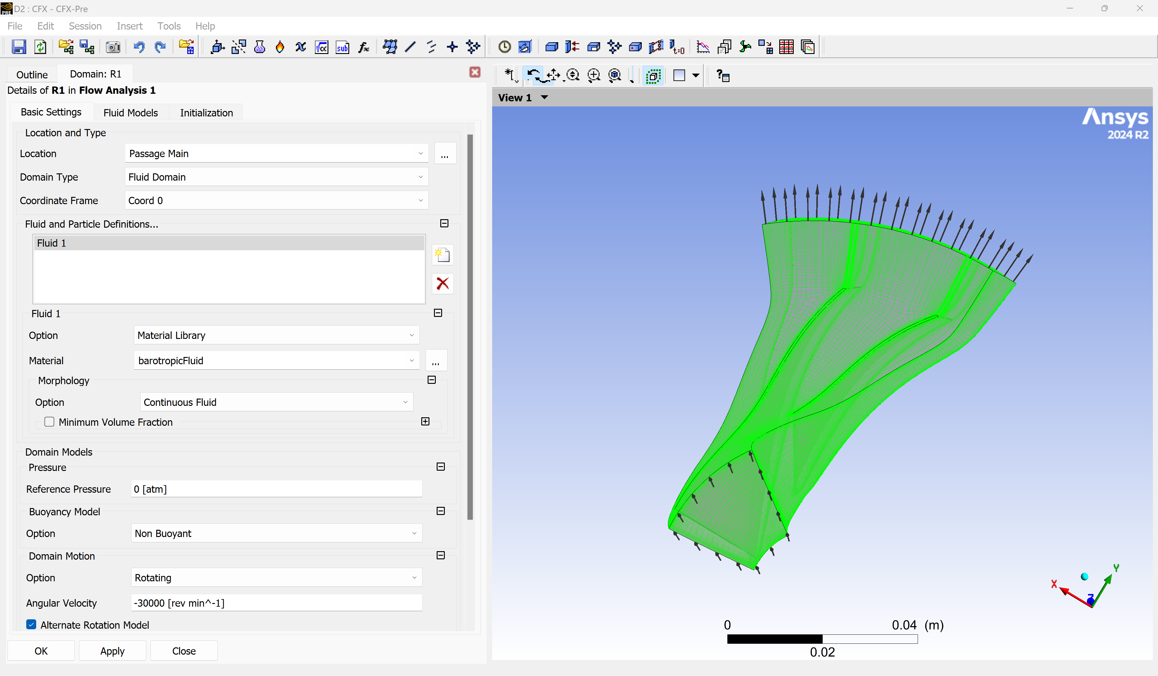
Step 3.5: Assign the barotropic fluid to the flow domain#

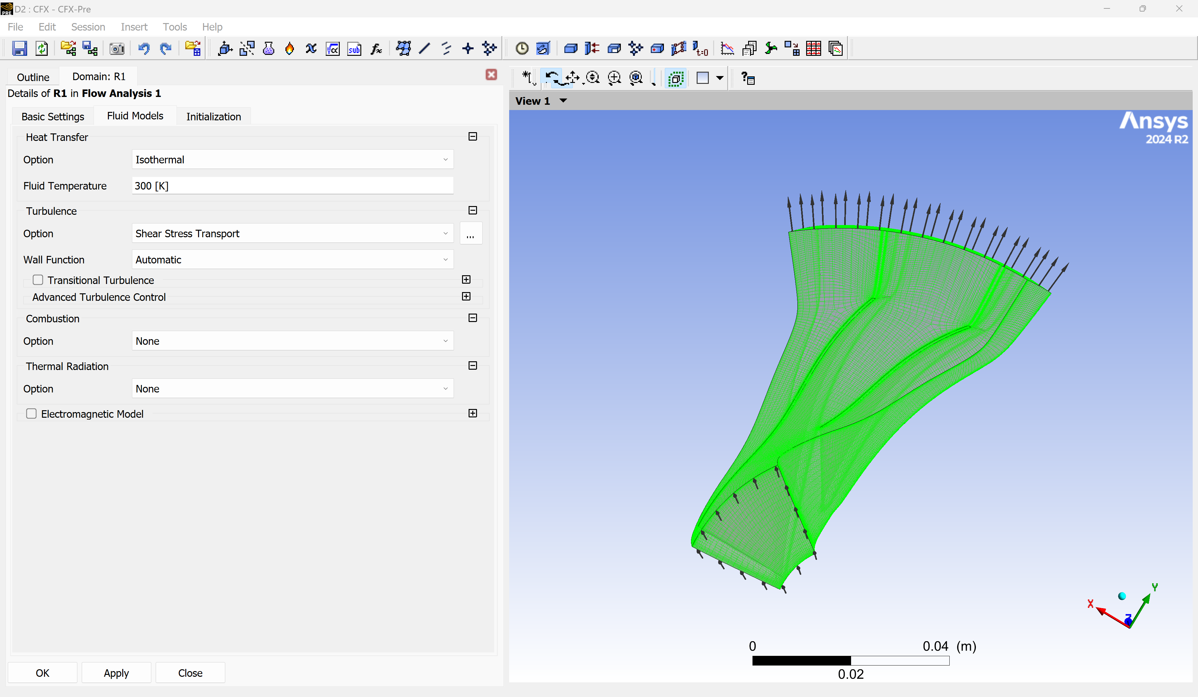
Go to the Simulation menu and open the settings for the flow domain R1 (which stands for Rotor 1).

In the Basic Settings tab, select barotropicFluid as the material and set the angular velocity of the domain.
In the Fluid Models tab, set Heat Transfer to Isothermal (this disables the energy equation) and choose your desired turbulence model.

CFX domain material and rotation CFX fluid model settings

Step 3.6: Define boundary conditions#

Open the “R1 Inlet” boundary and set the total pressure.

CFX inlet pressure

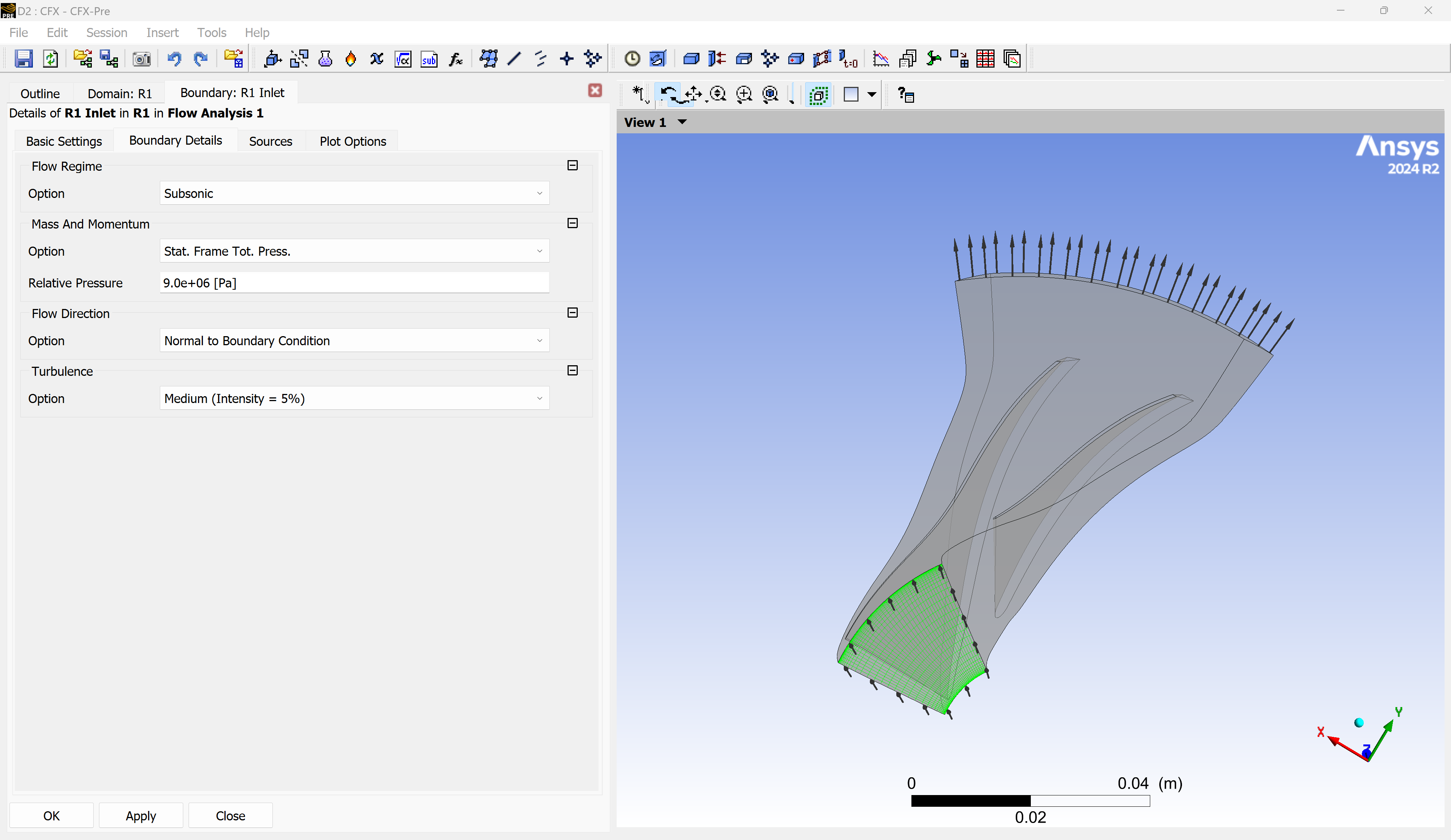
Then open the “R1 Outlet” boundary and define the mass flow rate. A value of 6.0 kg/s is selected to operate slightly below the choking condition for the given rotational speed, ensuring operation within the surge and choke margins.

CFX outlet mass flow

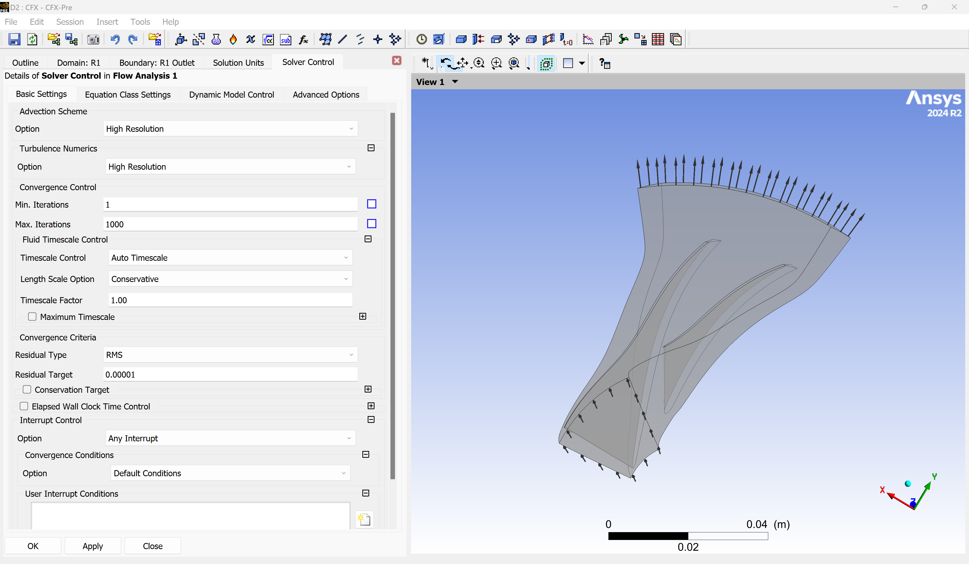
Step 3.7: Set solver parameters#

Go to the Solver Control section and open the Basic Settings tab.

Here, you can:

Select the discretization schemes for the flow and turbulence equations
Set the Timescale Factor to control the convergence speed toward a steady-state solution
Define the Residual Target for the simulation

The timescale should be chosen to ensure stable and efficient convergence.

Solver settings in CFX

Step 3.8: Run the simulation#

Save and close CFX Pre, then open the CFX Solver Manager.

Select the number of CPU cores and start the simulation.

alt text

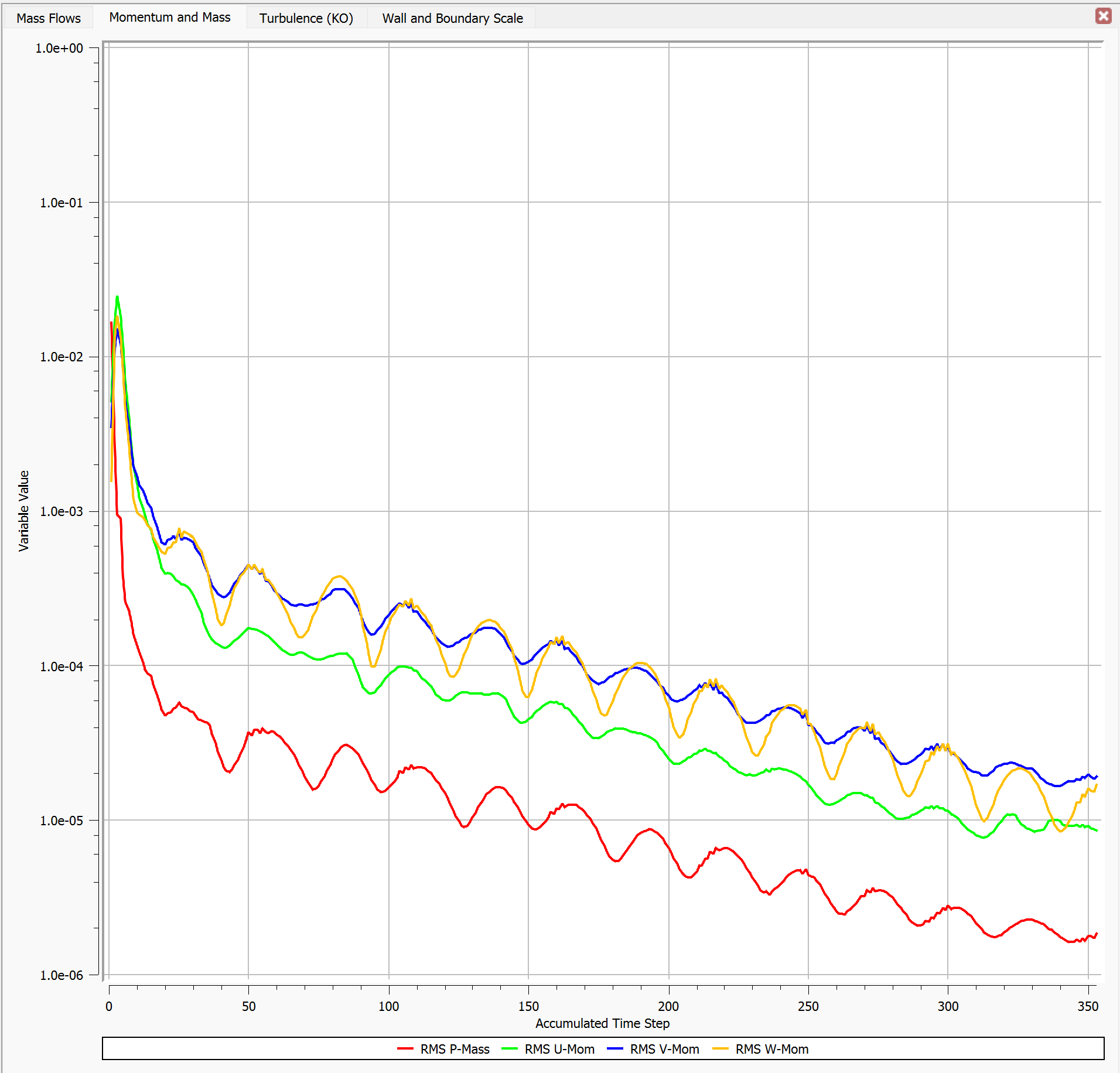
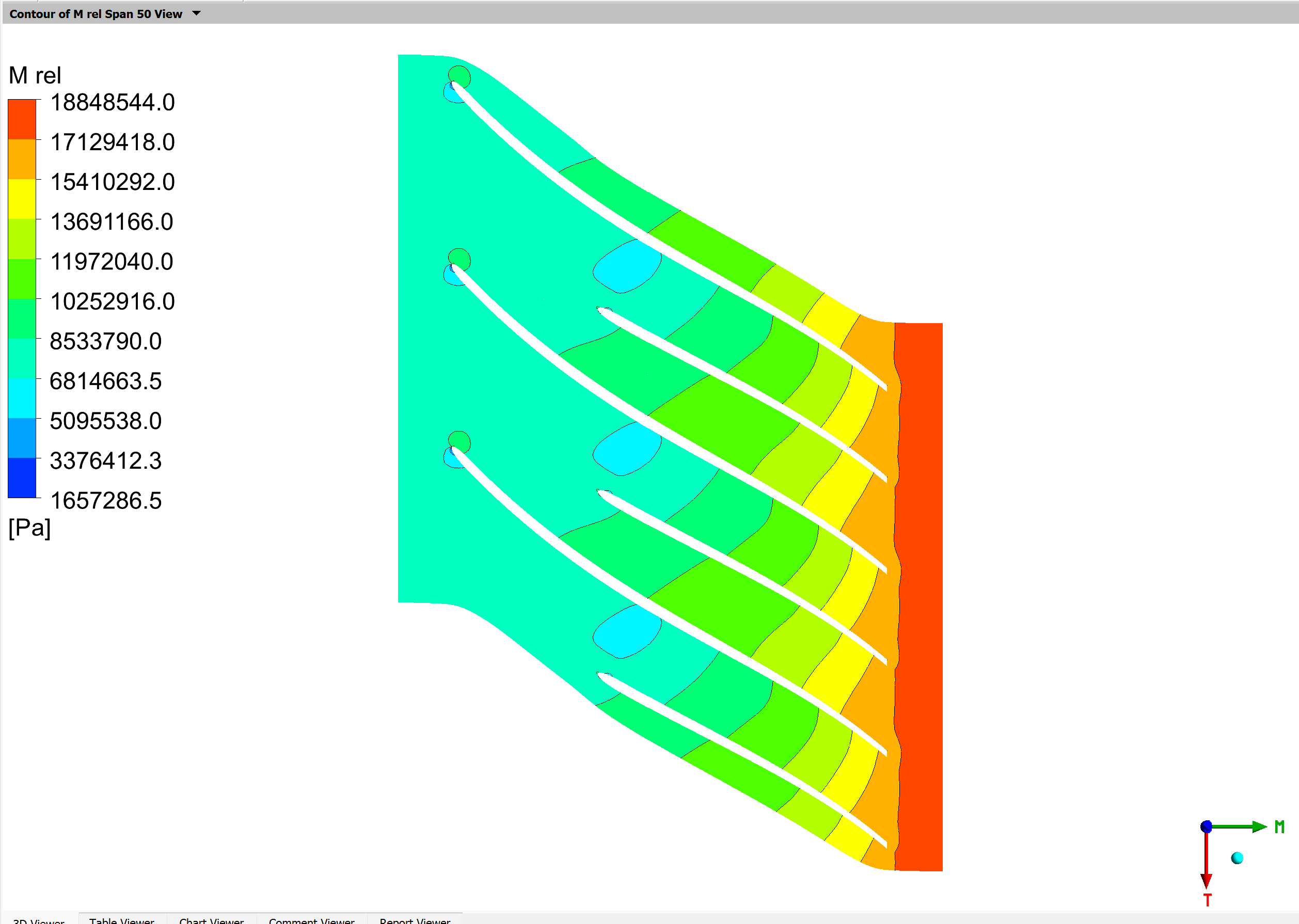
After convergence, open the results in CFD Post for visualization.

Note: The turbomachinery report in CFD Post may show errors. This is expected—since the barotropic model does not compute entropy or enthalpy, some predefined macros will fail. It does not affect the validity of the simulation.