Design optimization
This section guides you through the process of optimizing the design of axial turbines using TurboFlow. You will learn how to define optimization objectives, set constraints, and utilize the optimization algorithm to achieve the best design. Design optimization is excecuted in two steps:
Load configuration file.
Compute optimal turbine.
Illustrated by a code example:
import os
import turboflow as tf


CONFIG_FILE = os.path.abspath("my_configuration.yaml") # Get absolute path of configuration file
config = tf.load_config(CONFIG_FILE) # Load configuration file
solver = tf.compute_optimal_turbine(config, export_results=True) # Compute optimal turbine
This page describes the main functionalities and options available when designing turbines using turboflow:
Configuration setup
The configuration must be setup in a yaml file, where certain sections are required, while others are optional, meaning that a default value is provided. In the example below, the full configuration for design optimization is provided, where the required parts are marked with # required and the optional parts are marked with # optional.
In summary, these section are required:
turbomachinery : specifies the turbomachinery configuration.
operation_points: specifies the design point. If a list is provided, the first point is used.
The remaining input is optional. Here is an example of how the configuration file could look for a one-stage axial turbine:
turbomachinery: axial_turbine # Required
operation_points: # Required
    fluid_name: air # Required
    T0_in: 295.6 # Required
    p0_in: 13.8e4 # Required
    p_out : 13.8e4/2.298 # Required
    omega: 1627 # Required
    alpha_in: 0 # Required

simulation_options: # Optional
    deviation_model : aungier  # Optional
    choking_criterion : critical_mach_number # Optional
    rel_step_fd: 1e-4  # Optional
    loss_model:  # Optional
        model: benner  # Optional
        loss_coefficient: stagnation_pressure  # Optional
        inlet_displacement_thickness_height_ratio: 0.011  # Optional
        tuning_factors:  # Optional
            profile: 1.00  # Optional
            incidence: 1.00  # Optional
            secondary: 1.00  # Optional
            trailing: 1.00  # Optional
            clearance: 1.00  # Optional

design_optimization: # Optional
    objective_function: # Optional
        variable : overall.efficiency_ts # Optional
        scale : 10 # Optional
        type : maximize # Optional
    variables : # Optional
        specific_speed : # Optional
            value : 1.2
            lower_bound : 0.01
            upper_bound : 10
        blade_jet_ratio : # Optional
            value : 0.5
            lower_bound : 0.1
            upper_bound : 0.9
        hub_tip_ratio_in : # Optional
            value : [0.6, 0.6]
            lower_bound : [0.6, 0.6]
            upper_bound : [0.9, 0.9]
        hub_tip_ratio_out : # Optional
            value : [0.6, 0.6]
            lower_bound : [0.6, 0.6]
            upper_bound : [0.9, 0.9]
        aspect_ratio : # Optional
            value : [1.5, 1.5]
            lower_bound : [1.0, 1.0]
            upper_bound : [2.0, 2.0]
        pitch_chord_ratio : # Optional
            value : [0.9, 0.9]
            lower_bound : [0.75, 0.75]
            upper_bound : [1.10, 1.10]
        trailing_edge_thickness_opening_ratio : # Optional
            value : [0.1, 0.1]
            lower_bound : [0.05, 0.05]
            upper_bound : [0.4, 0.4]
        leading_edge_angle : # Optional
            value : [0.41, 0.5]
            lower_bound : [0.41, 0.08]
            upper_bound : [0.92, 0.58]
        gauging_angle : # Optional
            value : [0.17, 0.94]
            lower_bound : [0.06, 0.72]
            upper_bound : [0.28, 0.94]
        v_in : # Optional
            value : 0.1
            lower_bound : 0.001
            upper_bound : 0.5
        w_out : # Optional
            value : [0.65, 0.65]
            lower_bound : [0.1, 0.1]
            upper_bound : [1.0, 1.0]
        s_out : # Optional
            value : [0.15, 0.15]
            lower_bound : [0.0, 0.0]
            upper_bound : [0.32, 0.32]
        beta_out : # Optional
            value : [0.83, 0.17]
            lower_bound : [0.72, 0.06]
            upper_bound : [0.94, 0.28]
        v_crit_in : # Optional
            value : [0.4, 0.4]
            lower_bound : [0.1, 0.1]
            upper_bound : [1.0, 1.0]
        beta_crit_throat : # Optional
            value : [0.83, 0.17]
            lower_bound : [0.72, 0.06]
            upper_bound : [0.94, 0.28]
        w_crit_throat : # Optional
            value : [0.65, 0.65]
            lower_bound : [0.1, 0.1]
            upper_bound : [1.0, 1.0]
        s_crit_throat : # Optional
            value : [0.15, 0.15]
            lower_bound : [0.0, 0.0]
            upper_bound : [0.32, 0.32]
        throat_location_fraction : # Optional
            value : [1.0, 1.0]
            leading_edge_diameter :
            value : [2*0.127e-2, 2*0.081e-2]
        leading_edge_wedge_angle : # Optional
            value : [50.0, 50.0]
        tip_clearance : # Optional
            value : [0.00, 0.030e-2]
        cascade_type : # Optional
            value : ["stator", "rotor"]
    constraints : # Optional
        - variable : overall.mass_flow_rate  # Optional
          type : "="
          value : 2.5
          normalize : True
        - variable : additional_constraints.interspace_area_ratio  # Optional
          type : "="
          value : 1
          normalize : True
    radius_type : "constant_mean" # Optional
    solver_options: # Optional
        library: scipy # Optional
        method: slsqp # Optional
        derivative_method: 2-point # Optional
        derivative_abs_step: 1e-6 # Optional
        print_convergence: True # Optional
        plot_convergence: True # Optional
        update_on: "gradient" # Optional
        options : # Optional
            tol: 1e-3 # Optional
            max_iter: 100 # Optional
The design_optimization section contains information on the objective function, constraints and design variables:
objective_function: defined by specifying variable, type and scale.
constraints: each constraint is defined by specifying the variable name, type, value and if the constraint should be normalized or not.
variables: set of variables required for design optimization. The variable is considered a design variable if bounds are provided. All variables have a default value, and some have defualt bounds. Note that velocities (v and w), entropies (s) and flow angles (beta) must be design variables.
See Configuration Options for more information regarding the available inputs.
To load the configuration file, the absolute path must be provided to turboflow.load_config:
import os
import turboflow as tf


CONFIG_FILE = os.path.abspath("my_configuration.yaml") # Get absolute path of the configuration file
config = tf.load_config(CONFIG_FILE) # Load configuration file
Note
The only current available option for turbomachinery is axial_turbine.
Note
Velocities (v and w), entropies (s) and flow angles (beta) in the variables section must be provided with bounds (as design variables).
Compute optimal turbine
To compute the optimal turbine, simply provide the configuration file to the function compute_optimal_turbine:
import os
import turboflow as tf


CONFIG_FILE = os.path.abspath("my_configuration.yaml") # Get absolute path of the configuration file
config = tf.load_config(CONFIG_FILE) # Load configuration file
solver = tf.compute_optimal_turbine(
    out_filename=None,
    out_dir="output",
    export_results=True,
)
If export_results is set to True, the simulation data is exported as an Excel file. The file is saved either to a specified directory (out_dir) or to the default directory “output”. The default filename (out_filename) is design_optimization_{current_time}, where current_time is a string formatted as {year}{month}{day}{hour}{minute}_{second}.
Plotting results
Plotting functions are provided to graphically illustrate the simulated data:
Plot velocity triangles: turboflow.plot_velocity_triangles
Plot axial-radial plane: turboflow.plot_axial_radial_plane
Plot axial-tangential plane: turboflow.plot_view_axial_tangential
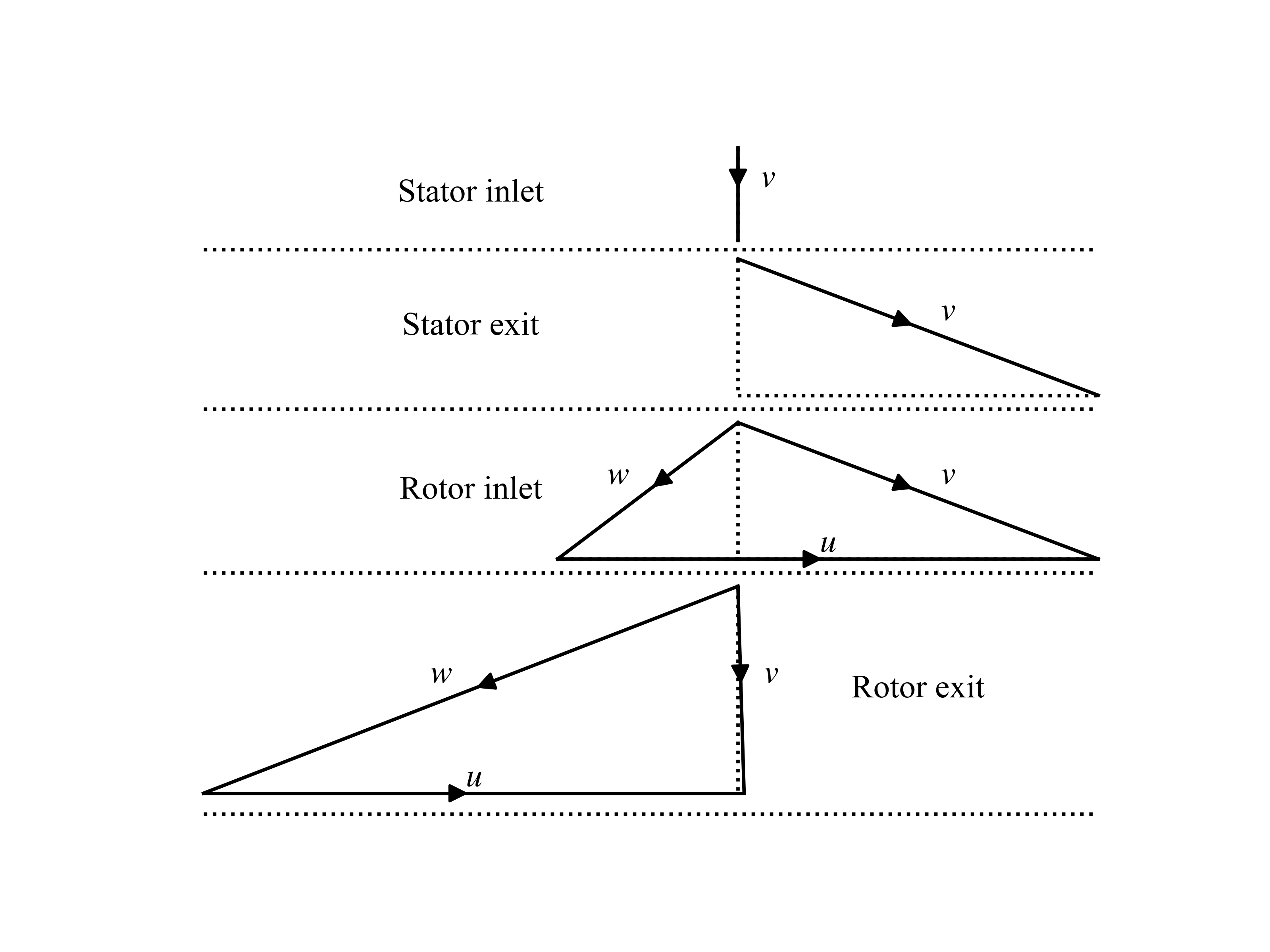
Plot velocity triangles
This function plots the velocity triangles at each plane of the axial turbine. The plot is initialized by providing the plane specific data from the solution of optimization problem:
import os
import turboflow as tf


CONFIG_FILE = os.path.abspath("my_configuration.yaml") # Get absolute path of the configuration file
config = tf.load_config(CONFIG_FILE) # Load configuration file
solver = tf.compute_optimal_turbine(
    out_filename=None,
    out_dir="output",
    export_results=True,
)

fig, ax = tf.plot_functions.plot_velocity_triangles_planes(solver.problem.results["plane"])
Here is an example of how the velocity triangle plots looks:
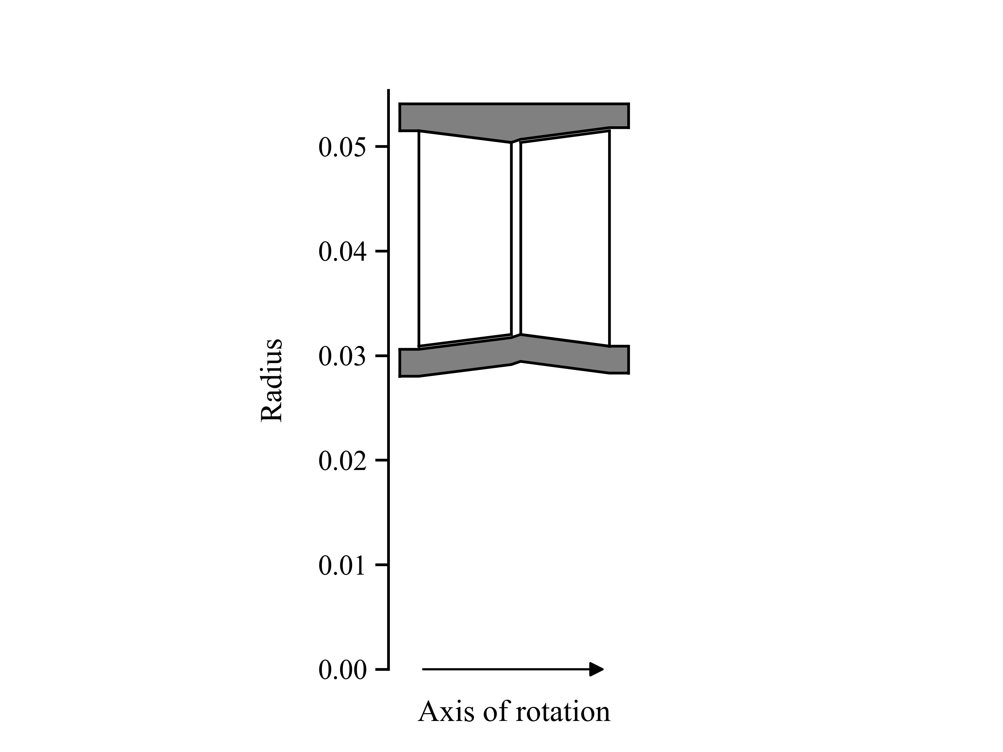
Plot axial-radial plane
This function plots the geometry of an axial-turbine in the axial-radial plane. The plot is initialized by providing the geometry from the solution of the optimization problem:
import os
import turboflow as tf


CONFIG_FILE = os.path.abspath("my_configuration.yaml") # Get absolute path of the configuration file
config = tf.load_config(CONFIG_FILE) # Load configuration file
solver = tf.compute_optimal_turbine(
    out_filename=None,
    out_dir="output",
    export_results=True,
)

fig, ax = tf.plot_functions.plot_axial_radial_plane(solver.problem.geometry)
Here is an example of how the plot look:
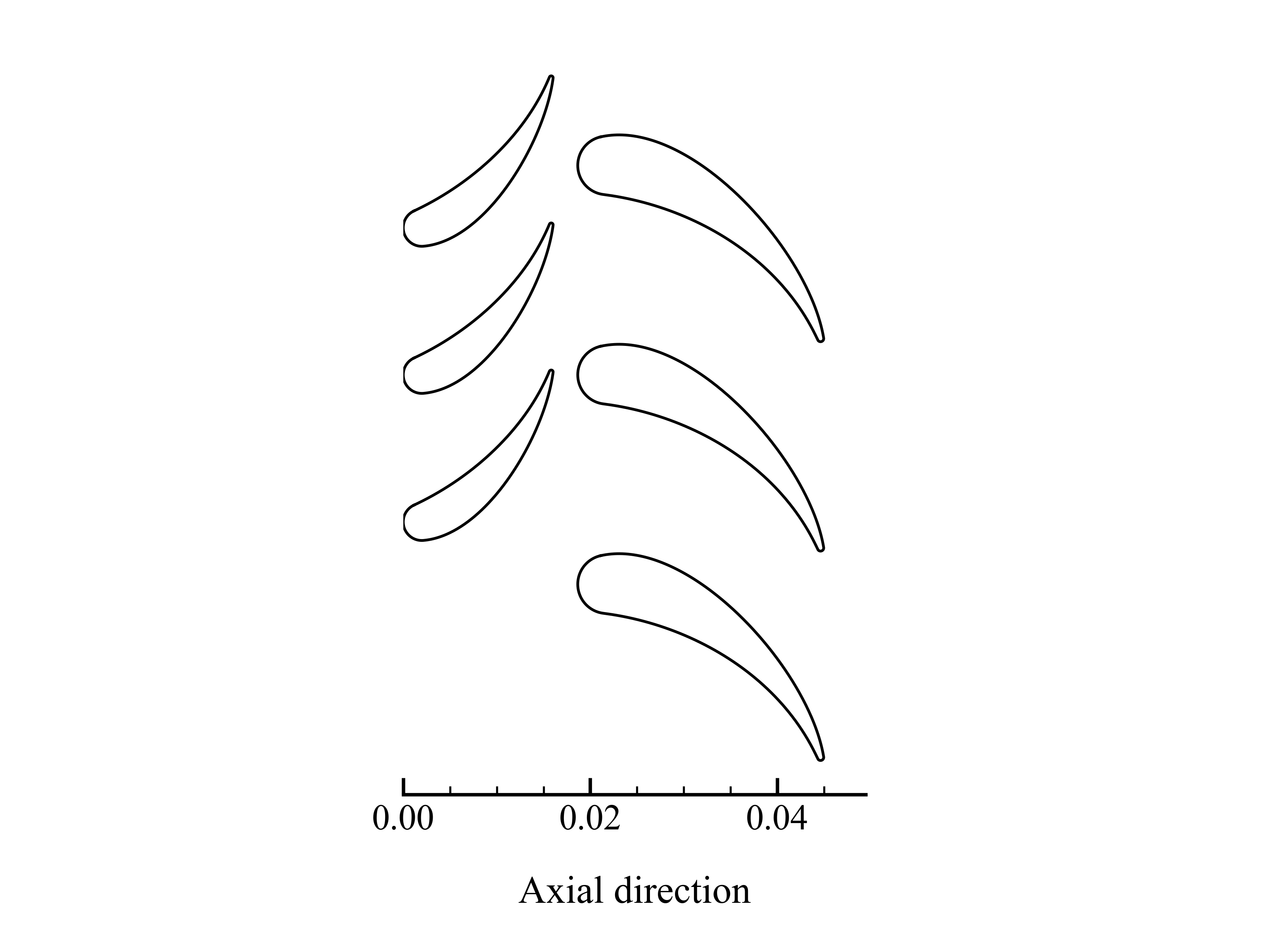
Plot axial-tangential plane
This function plots the geometry of an axial-turbine in the axial-tangential plane. The plot is initialized by providing a solver object:
import os
import turboflow as tf

CONFIG_FILE = os.path.abspath("my_configuration.yaml") # Get absolute path of the configuration file
config = tf.load_config(CONFIG_FILE) # Load configuration file
solver = tf.compute_optimal_turbine(
    out_filename=None,
    out_dir="output",
    export_results=True,
)

# Plot geometry in the axial-tangential plane
fig, ax = tf.plot_functions.plot_view_axial_tangential(solver.problem)
Here is an example of how the plot look: