Performance prediction
In this section, you will learn how to use TurboFlow to predict the performance of axial turbines. This includes setting up the configuration file, running the analysis, and interpreting the results. Performance prediction is excecuted in three steps:
Load configuration file.
Define operating points where the turbine should be evaluated.
Compute performance.
Illustrated by a code example:
import os
import turboflow as tf


CONFIG_FILE = os.path.abspath("my_configuration.yaml") # Get absolute path of configuration file
config = tf.load_config(CONFIG_FILE) # Load configuration file
operation_points = config["operation_points"] # Define operating points
solvers = tf.compute_performance(
    operation_points,
    config,
    export_results=True,
    stop_on_failure=True,
) # Evaluate turbine
This page describes the main functionalities and options available when simulating performance of axial turbines:
Configuration setup
The configuration must be setup in a yaml file, where certain sections are required, while others are optional, meaning that a default value is provided. In the example below, the full configuration for performance prediction is provided, where the required parts are marked with # required and the optional parts are marked with # optional. Note that to simulate performance across a perfomance map, the performance_map section is also required.
In summary, these section are required:
turbomachinery : specifies the turbomachinery configuration.
geometry: all necessary geometrical variables.
operation_points: operational points at which the turbine should be evaluated.
while the rest is optional. Here is an example of how the confiugration file could look for a one-stage axial turbine:
turbomachinery: axial_turbine # Required
operation_points: # Required
    fluid_name: air # Required
    T0_in: 295.6 # Required
    p0_in: 13.8e4 # Required
    p_out : 13.8e4/2.298 # Required
    omega: 1627 # Required
    alpha_in: 0 # Required

simulation_options: # Optional
    deviation_model : aungier  # Optional
    choking_criterion : critical_mach_number # Optional
    rel_step_fd: 1e-4  # Optional
    loss_model:  # Optional
        model: benner  # Optional
        loss_coefficient: stagnation_pressure  # Optional
        inlet_displacement_thickness_height_ratio: 0.011  # Optional
        tuning_factors:  # Optional
            profile: 1.00  # Optional
            incidence: 1.00  # Optional
            secondary: 1.00  # Optional
            trailing: 1.00  # Optional
            clearance: 1.00  # Optional

performance_analysis : # Optional
    performance_map: # Required if simulating performance across performance map
        fluid_name: air
        T0_in: 295.6
        p0_in: 13.8e4
        p_out: 13.8e4/np.linspace(1.6, 4.5, 40)
        omega: 1627
        alpha_in: 0
    solver_options: # Optional
        method: hybr  # Optional
        tolerance: 1e-8  # Optional
        max_iterations: 100  # Optional
        derivative_method: "2-point"  # Optional
        derivative_abs_step: 1e-6  # Optional
        print_convergence: True # Optional
        plot_convergence: False # Optional
    initial_guess :
        efficiency_tt : [0.9, 0.8]
        efficiency_ke : [0.2, 0.1]
        ma_1 : [0.8, 0.8]
        ma_2 : [0.8, 0.8]

geometry: # Required
    cascade_type: ["stator", "rotor"] # Required
    radius_hub_in: [0.084785, 0.084785] # Required
    radius_hub_out: [0.084785, 0.081875] # Required
    radius_tip_in: [0.118415, 0.118415] # Required
    radius_tip_out: [0.118415, 0.121325] # Required
    pitch: [1.8294e-2, 1.524e-2] # Required
    chord: [2.616e-2, 2.606e-2] # Required
    stagger_angle: [+43.03, -31.05] # Required
    opening: [0.747503242e-2, 0.735223377e-2] # Required
    leading_edge_angle : [0.00, 29.60] # Required
    leading_edge_wedge_angle : [50.00, 50.00] # Required
    leading_edge_diameter : [2*0.127e-2, 2*0.081e-2] # Required
    trailing_edge_thickness : [0.050e-2, 0.050e-2] # Required
    maximum_thickness : [0.505e-2, 0.447e-2] # Required
    tip_clearance: [0.00, 0.030e-2] # Required
    throat_location_fraction: [1, 1] # Required
To load the configuration file, the absolute path must be provided to turboflow.load_config:
import os
import turboflow as tf


CONFIG_FILE = os.path.abspath("my_configuration.yaml") # Get absolute path of the configuration file
config = tf.load_config(CONFIG_FILE) # Load configuration file
Note
The only current available option for turbomachinery is axial_turbine.
Compute performance at a single point
To perform single-point performance prediction, the operation_points section in the configuration file should be defined in the following way:
operation_points:
    fluid_name: air
    T0_in: 295.6
    p0_in: 13.8e4
    p_out : 13.8e4/2.0
    omega: 1627
    alpha_in: 0
After loading the configuration file, the operation point is extracted from the configuration file, and provided to turboflow.compute_performance:
import os
import turboflow as tf


CONFIG_FILE = os.path.abspath("my_configuration.yaml")
config = tf.load_config(CONFIG_FILE) # Load configuration file
operation_points = config["operation_points"] # Extract operation point
solvers = tf.compute_performance(
    operation_points,
    config,
    export_results=True,
    stop_on_failure=True,
) # Compute performance at operation point
Compute performance at a set of points
To perform performance prediction at a set of operation points, the operation_points section in the configuration file should be a list of operating points:
operation_points:
    - fluid_name: air # First point
      T0_in: 295.6
      p0_in: 13.8e4
      p_out : 13.8e4/2.0
      omega: 1627
      alpha_in: 0
    - fluid_name: air # Second point
      T0_in: 295.6
      p0_in: 13.8e4
      p_out : 13.8e4/3.0
      omega: 1627
      alpha_in: 0
After loading the configuration file, the operation points are extracted from the configuration file, and provided to turboflow.compute_performance:
import os
import turboflow as tf


CONFIG_FILE = os.path.abspath("my_configuration.yaml")
config = tf.load_config(CONFIG_FILE) # Load configuration file
operation_points = config["operation_points"] # Extract operation points
solvers = tf.compute_performance(
    operation_points,
    config,
    export_results=True,
    stop_on_failure=True,
) # Compute performance at operation points
Compute performance across a performance map
To perform performance prediction across a performance map, a perfomance_map section must be defined within the performance_analysis section:
performance_analysis :
  performance_map:
      fluid_name: air
      T0_in: 295.6
      p0_in: 13.8e4
      p_out: 13.8e4/np.linspace(1.6, 4.5, 40)
      omega: 1627*np.array([0.9, 1.0, 1.1])
      alpha_in: 0
The performance map is defined by setting either a value or a range for each boundary condition. The perfomance map is constructed by generating a list of every combination of the given values/ranges. In the example above, the performance will be simulated for a total-to-static pressure ratio between 1.6 and 4.5 at 90%, 100% and 110% of the design angular speed (omega = 1627).
After loading the configuration file, the performance map is extracted from the configuration file, and provided to turboflow.compute_performance:
import os
import turboflow as tf


CONFIG_FILE = os.path.abspath("my_configuration.yaml")
config = tf.load_config(CONFIG_FILE) # Load configuration file
operation_points = config["performance_analysis"]["performance_map"] # Extract perfomance map
solvers = tf.compute_performance(
    operation_points,
    config,
    export_results=True,
    stop_on_failure=True,
) # Compute performance at operation points
Export results
When calling turboflow.compute_performance(), there are some keyword arguments available:
solvers = tf.compute_performance(
    operation_points,
    config,
    export_results=True,
    out_dir = "output",
    out_filename = None,
    stop_on_failure=False,
)
If export_results is set to True, the simulation data is exported as an Excel file. The file is saved either to a specified directory (out_dir) or to the default directory “output”. The default filename (out_filename) is performance_analysis_{current_time}, where current_time is a string formatted as {year}{month}{day}{hour}{minute}_{second}.
The stop_on_failure breaks the analysis if one of the operation points fails to converge.
Plotting results
Plotting functions are provided to graphically illustrate the simulated data. It supports various types of plots, including:
Plot single line, e.g. mass flow rate as a function of pressure ratio
Plot several lines, e.g. mass flow rate as a function of pressure ratio at sifferent rotational speed
Stacked plots, e.g. stacked loss coefficients as a function of pressure ratio
The first three types are made by loading the Excel file with the simulated data, and specify the x and y parameter in the plot (x_key and y_key):
import turboflow as tf
import matplotlib.pyplot as plt

filename = "output/performance_analysis_2024-01-01_01-01-01.xlsx"
data = tf.plot_functions.load_data(filename) # Load results data

fig1, ax1 = tf.plot_functions.plot_lines(
    data, # datset
    x_key="PR_ts", # x-axis key
    y_keys=["mass_flow_rate"], # y-axis key
    xlabel="Total-to-static pressure ratio", # axis x-label
    ylabel="Mass flow rate [kg/s]", # axis y-label
    title="Turbine mass flow rate", # axis title
    filename="mass_flow_rate", # filename if figure should be saved
    outdir="figures", # output directory if figure should be saved
    save_figs=True,
)

plt.show()
The subsequent subsections gives a more detailed description of how to setup up the various plots.
Plot single line
To plot a single line, simply specify the list y_keys with one key:
import turboflow as tf
import matplotlib.pyplot as plt

filename = "output/performance_analysis_2024-01-01_01-01-01.xlsx"
data = tf.plot_functions.load_data(filename) # Load results data

fig1, ax1 = tf.plot_functions.plot_lines(
    data, # datset
    x_key="PR_ts", # x-axis key
    y_keys=["mass_flow_rate"], # y-axis key
    xlabel="Total-to-static pressure ratio", # axis x-label
    ylabel="Mass flow rate [kg/s]", # axis y-label
    title="Turbine mass flow rate", # axis title
    filename="mass_flow_rate", # filename if figure should be saved
    outdir="figures", # output directory if figure should be saved
    save_figs=True,
)

plt.show()
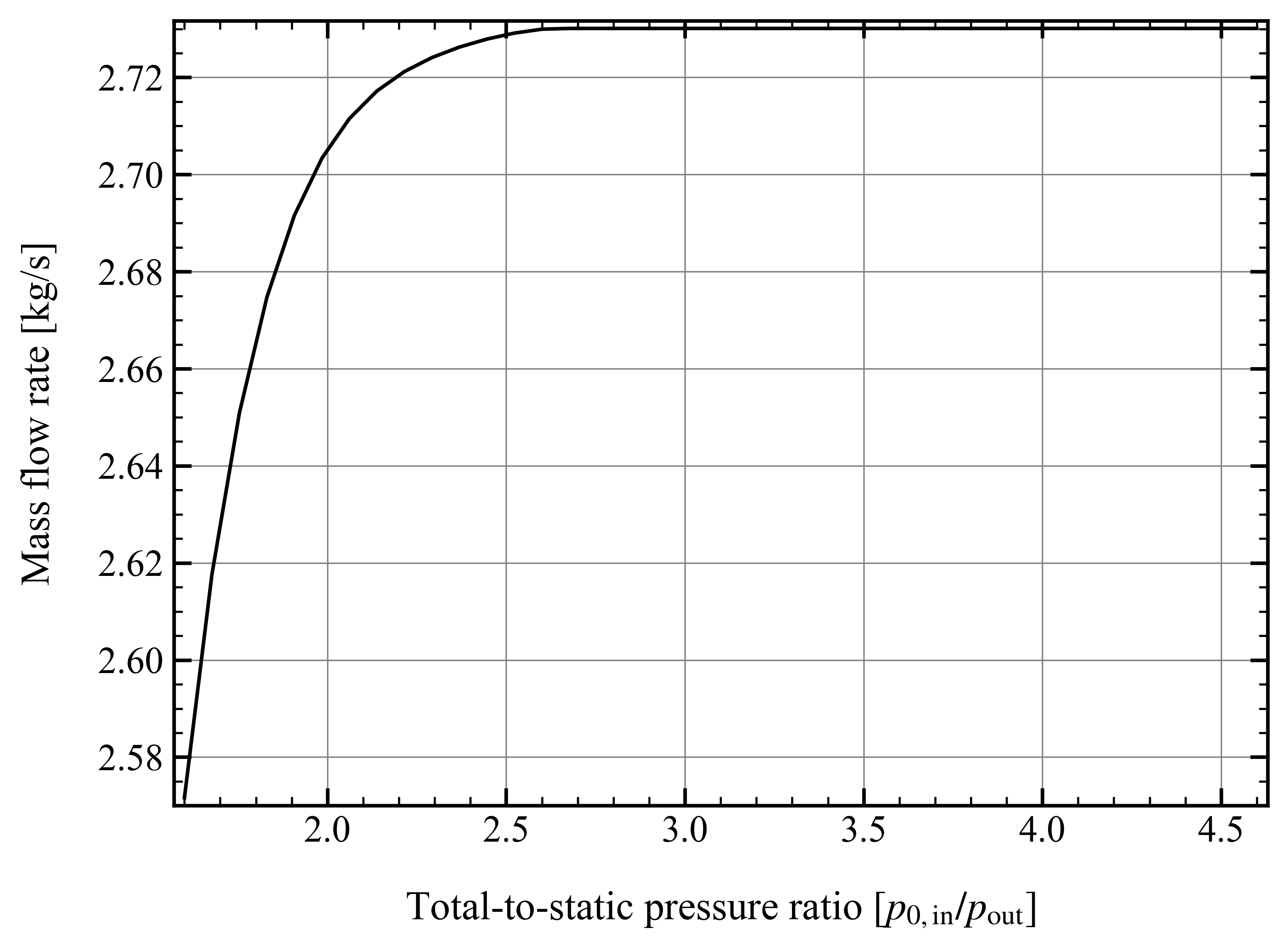
Note that if the excel file contain a whole performance map (e.g. a range of pressure ratios and angular speed), it is convenient to filter out a subset of this file (e.g. results at one specific angular speed). Here is an example, where the data is filtered based on a specific angular speed:
import turboflow as tf
import matplotlib.pyplot as plt

filename = "output/performance_analysis_2024-01-01_01-01-01.xlsx"
data = tf.plot_functions.load_data(filename) # Load results data

# Plot mass flow rate
subsets = ["omega", 1627]
fig1, ax1 = tf.plot_functions.plot_lines(
    data,
    x_key="PR_ts",
    y_keys=["mass_flow_rate"],
    subsets=subsets,
    xlabel="Total-to-static pressure ratio [$p_{0, \mathrm{in}}/p_\mathrm{out}$]",
    ylabel="Mass flow rate [kg/s]",
    colors='k',
    filename = 'design_speed_mass_flow_rate',
    outdir = "figures",
    save_figs=True,
)

plt.show()
subsets is used to filter a subset of the original dataset. It is constructed as a list, where the first element is a string that specifies the parameter you want to use to filter the data. The subsequent elements are the values of the selected parameter that you want to include in your subset.
The example above would give the following figure:
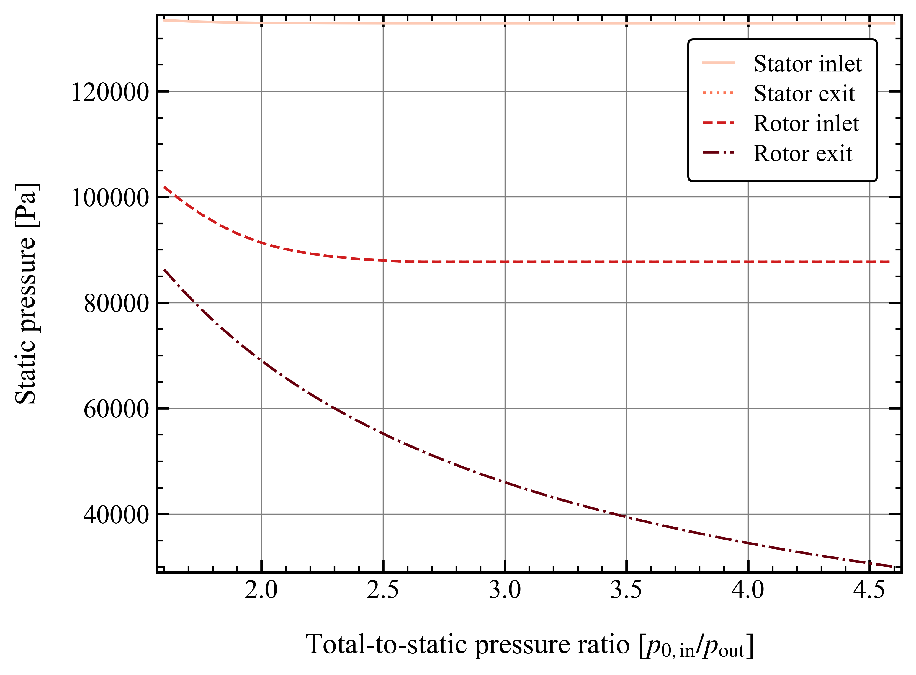
Plot several lines
To plot several lines, To plot a single line, simply specify the list y_keys with several keys:
import turboflow as tf
import matplotlib.pyplot as plt

filename = "output/performance_analysis_2024-01-01_01-01-01.xlsx"
data = tf.plot_functions.load_data(filename) # Load results data

# Plot mass flow rate
subset = ["omega", 1627]
labels = ["Stator inlet", "Stator exit", "Rotor inlet", "Rotor exit"]
fig1, ax1 = tf.plot_functions.plot_lines(
    data,
    x_key="PR_ts",
    y_keys=["p_1", "p_2", "p_3", "p_4"],
    subsets = subset,
    xlabel="Total-to-static pressure ratio [$p_{0, \mathrm{in}}/p_\mathrm{out}$]",
    ylabel="Static pressure [Pa]",
    linestyles=["-", ":", "--", "-."],
    color_map='Reds',
    labels = labels,
    filename='static_pressure',
    outdir = "figures",
    save_figs=True,
)

plt.show()
This example would give the following figure:
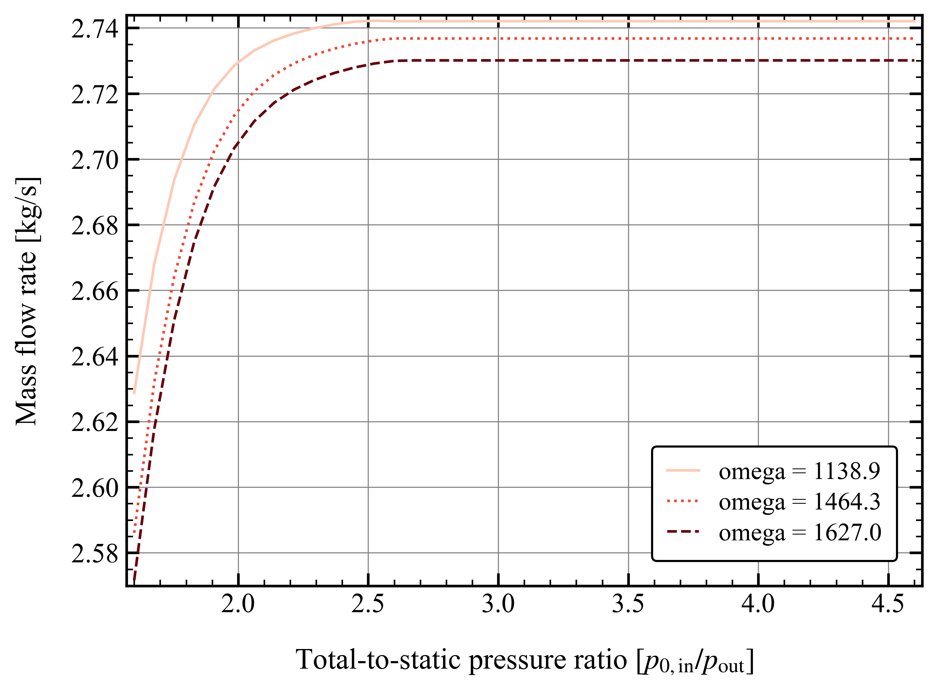
Similarly for the single point line, a subset can be defined. However, you can define several subsets, by specifying more values for the selected parameter. In this example, the mass flow rate is plotted as a function of total-to-static pressure ratio, at different subsets of angular speed:
import turboflow as tf
import matplotlib.pyplot as plt
import numpy as np

filename = "output/performance_analysis_2024-01-01_01-01-01.xlsx"
data = tf.plot_functions.load_data(filename) # Load results data

# Plot mass flow rate
subsets = ["omega"] + list(np.array([0.7, 0.9, 1])*1627)
fig1, ax1 = tf.plot_functions.plot_lines(
    data,
    x_key="PR_ts",
    y_keys=["mass_flow_rate"],
    subsets=subsets,
    xlabel="Total-to-static pressure ratio [$p_{0, \mathrm{in}}/p_\mathrm{out}$]",
    ylabel="Mass flow rate [kg/s]",
    linestyles=["-", ":", "--"],
    color_map='Reds',
    filename = 'mass_flow_rate',
    outdir = "figures",
    save_figs=True,
)

plt.show()
resulting in this figure:
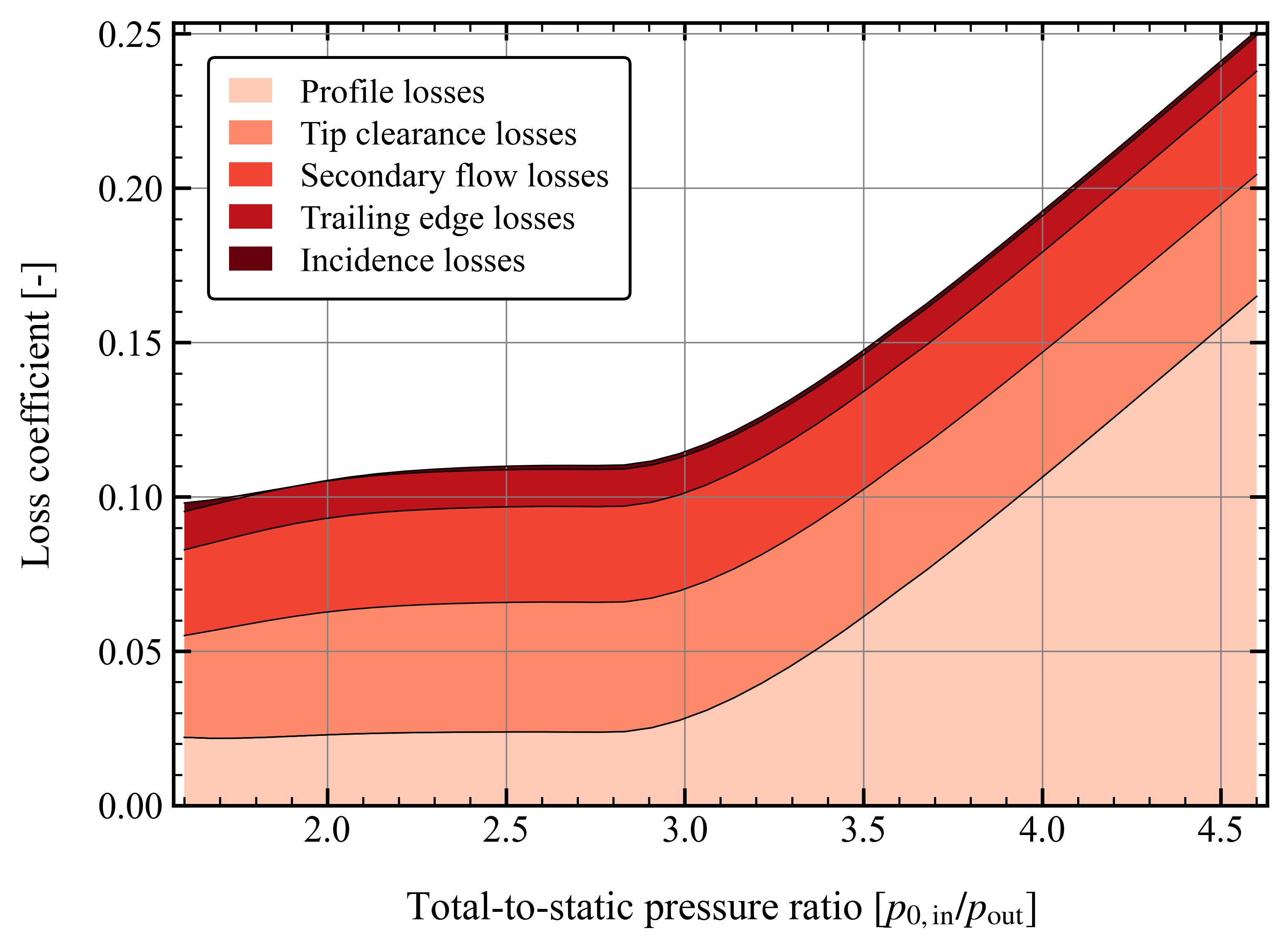
Stacked plots
Stacked plots can be convenient to illustrate the different loss coefficients at different operating points. Stacked plots are made by specifying stack = True
import turboflow as tf
import matplotlib.pyplot as plt

filename = "output/performance_analysis_2024-01-01_01-01-01.xlsx"
data = tf.plot_functions.load_data(filename) # Load results data

# Plot mass flow rate
subset = ["omega"] + [1627]
labels = ["Profile losses", "Tip clearance losses", "Secondary flow losses", "Trailing edge losses", "Incidence losses"]
fig1, ax1 = tf.plot_functions.plot_lines(
    data,
    x_key="PR_ts",
    y_keys=[
        "loss_profile_4",
        "loss_clearance_4",
        "loss_secondary_4",
        "loss_trailing_4",
        "loss_incidence_4",
    ],
    subsets = subset,
    xlabel="Total-to-static pressure ratio [$p_{0, \mathrm{in}}/p_\mathrm{out}$]",
    ylabel="Loss coefficient [-]",
    color_map='Reds',
    labels = labels,
    stack=True,
    filename="loss_coefficients",
    outdir="figures",
    save_figs = True,
)

plt.show()
This would result in this figure:
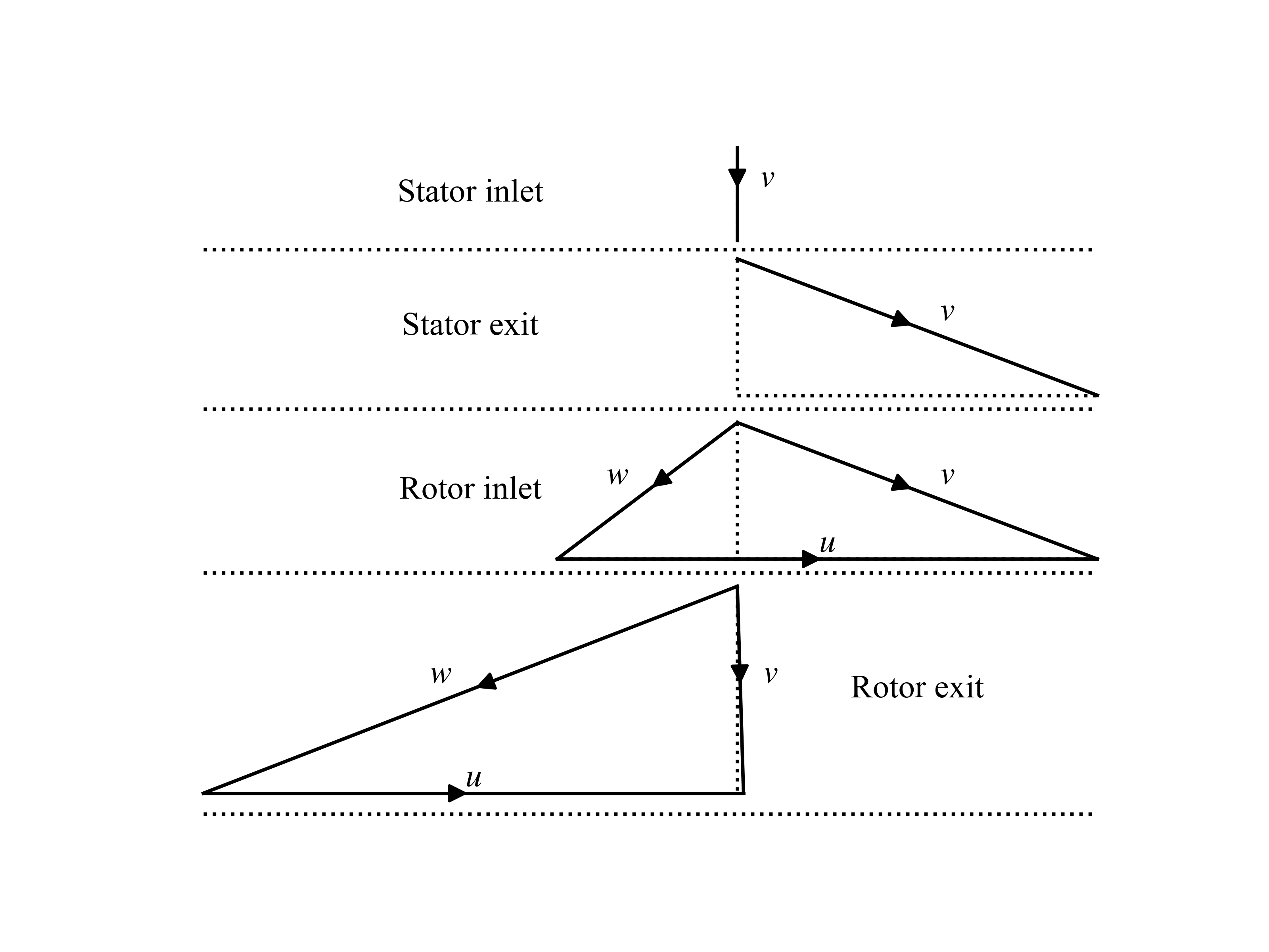
Plot velocity triangles
This function plots the velocity triangles of an axial-turbine for a certain operation point. The plot is initialized by providing a solver object:
import os
import turboflow as tf

# Perform analysis
CONFIG_FILE = os.path.abspath("my_configuration.yaml") # Get absolute path of the configuration file
config = tf.load_config(CONFIG_FILE) # Load configuration file
solvers = tf.compute_performance(
    operation_points,
    config,
)

# PLot velocity triangles
fig, ax = tf.plot_functions.plot_axial_radial_plane(solvers[0].problem.geometry)
Here is an example of how the velocity triangle plots looks:
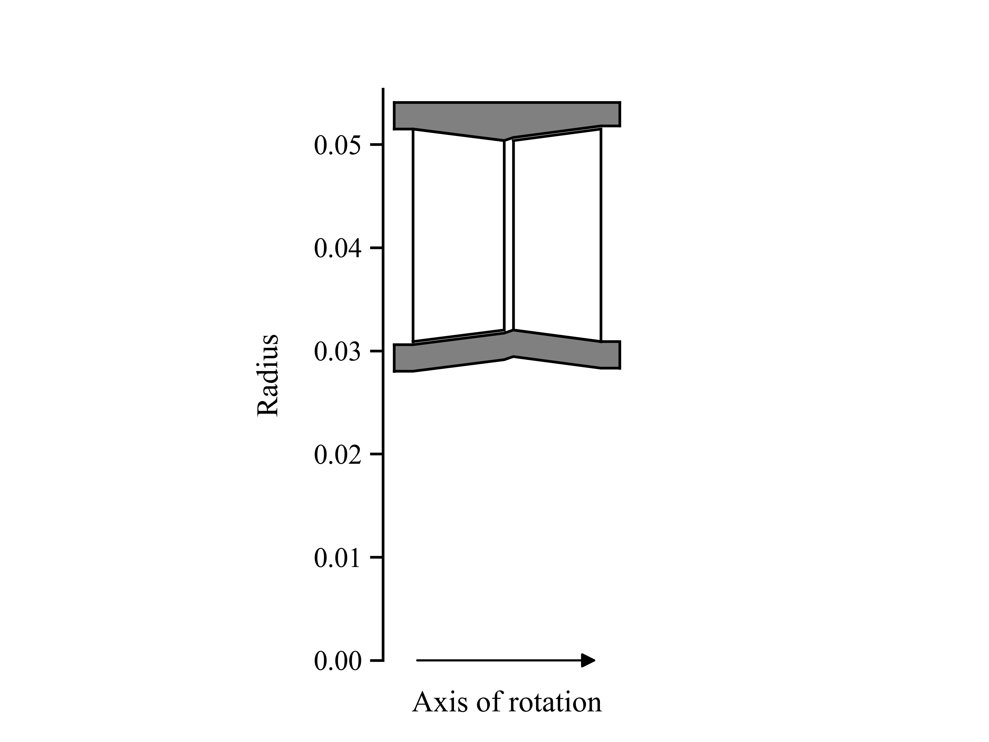
Plot axial-radial plane
This function plots the geometry of an axial-turbine in the axial-radial plane. The plot is initialized by providing a solver object:
import os
import turboflow as tf

# Perform analysis
CONFIG_FILE = os.path.abspath("my_configuration.yaml") # Get absolute path of the configuration file
config = tf.load_config(CONFIG_FILE) # Load configuration file
solvers = tf.compute_performance(
    operation_points,
    config,
)

# Plot geometry in the axial-radial plane
fig, ax = tf.plot_functions.plot_velocity_triangles_planes(solvers[0].problem.results["plane"])
Here is an example of how the plot look:
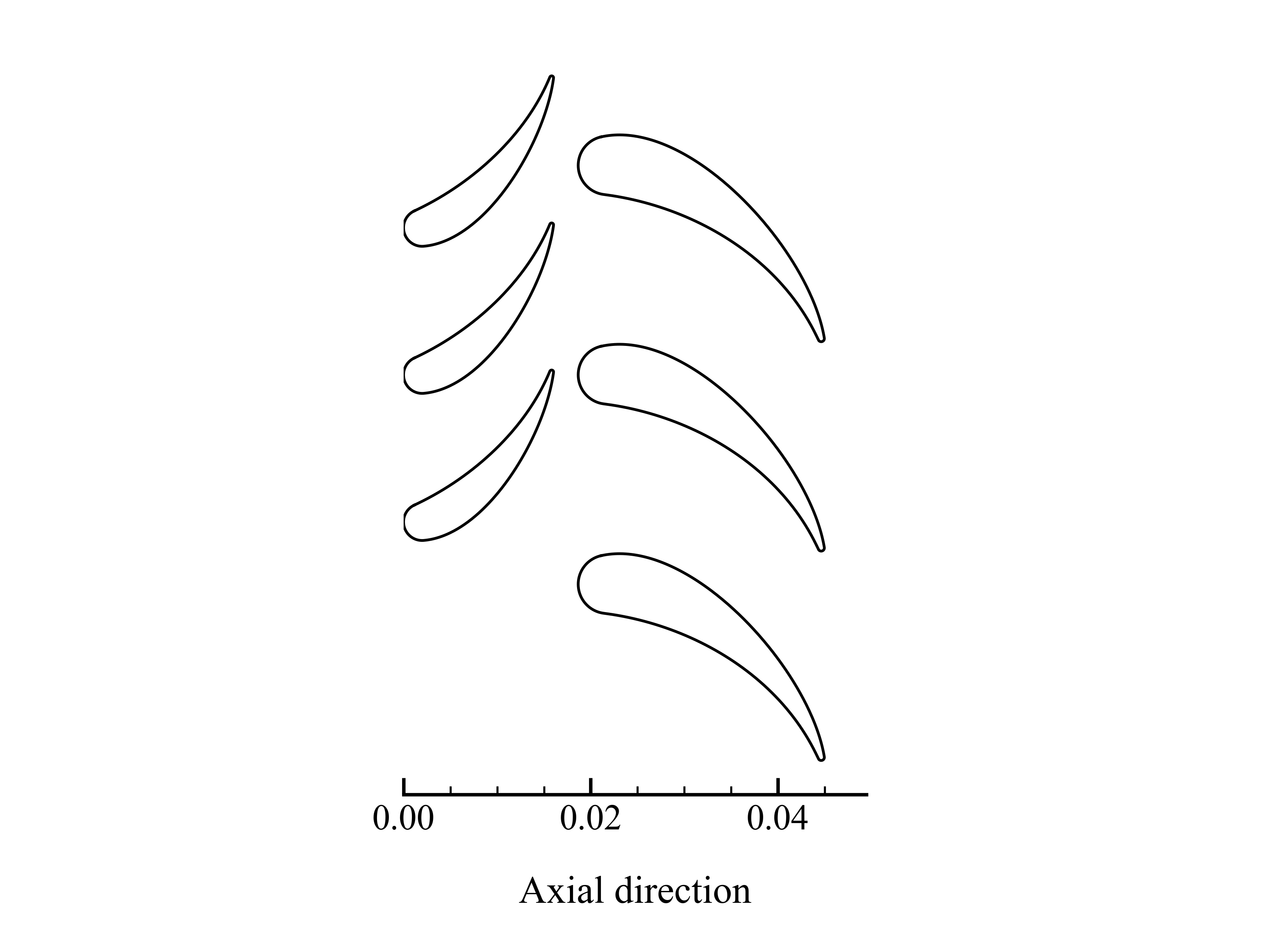
Plot axial-tangential plane
This function plots the geometry of an axial-turbine in the axial-tangential plane. The plot is initialized by providing a solver object:
import os
import turboflow as tf

# Perform analysis
CONFIG_FILE = os.path.abspath("my_configuration.yaml") # Get absolute path of the configuration file
config = tf.load_config(CONFIG_FILE) # Load configuration file
solvers = tf.compute_performance(
    operation_points,
    config,
)

# Plot geometry in the axial-tangential plane
fig, ax = tf.plot_functions.plot_view_axial_tangential(solvers[0].problem)
Here is an example of how the plot look: