Design a two-phase nozzle

This example designs a symmetric nozzle for nitrogen starting as subcooled liquid, using the flashing case in Cioffi et al. [2026]. You will set the inlet state, solve the expansion, inspect the characteristic mesh and flow properties, and export the two walls.

Configure the expansion

Input	Value	Meaning
fluid_name	"nitrogen"	Fluid used by the thermodynamic model.
P0	20e5 Pa	Stagnation pressure of 20 bar.
T0	\(T_\mathrm{sat}(20\,\mathrm{bar})-10\) K	Liquid inlet with 10 K subcooling.
p_back	2e5 Pa	Target back pressure of 2 bar.
solver	"conventional"	Nozzle solver with a rounded expansion section.

The script computes saturation temperature from CoolProp and subtracts the specified subcooling. Pressure and temperature define this single-phase inlet; quality is not supplied. The expansion subsequently enters the two-phase region. The default throat half-height is 0.01 m. The example checks convergence before plotting or exporting the wall.

Run and inspect the script

Run from the repository root after following the source installation instructions:

poetry run python examples/moc_design/nozzle_design.py

The code below is included directly from the example. The final display block is omitted; the script opens the figures with plt.show() during normal runs.

from pathlib import Path

import matplotlib.pyplot as plt
import numpy as np
from CoolProp.CoolProp import PropsSI

import turbo_moc
from turbo_moc.reporting import logging_context

# 1. Nitrogen flashing case from Cioffi et al. (NICFD 2026), Fig. 2:
#    20 bar stagnation pressure and 10 K inlet subcooling, expanding to 2 bar.
P0 = 20e5
T0 = PropsSI("T", "P", P0, "Q", 0, "Nitrogen") - 10.0
# Show the solver's progress on the console (INFO; use level="DEBUG" for details).
with logging_context():
    data = turbo_moc.design_nozzle(
        fluid_name="nitrogen",
        P0=P0,  # Stagnation pressure [Pa].
        T0=T0,  # Subcooled-liquid inlet temperature [K]; quality is not specified.
        p_back=2e5,  # Back pressure [Pa].
        solver="conventional",
    )

if not data["converged"] or not data["wall_final"]["x"]:
    raise RuntimeError("The nozzle design did not converge.")

wall = data["wall_final"]

# Plotting helpers return (figure, axes); keep the figures for SVG export.
figures = {
    "nozzle_contour": turbo_moc.mpl.plot_nozzle_contour(data)[0],
    "characteristics_mesh": turbo_moc.mpl.plot_characteristics_mesh(data)[0],
    "axis_properties": turbo_moc.mpl.plot_axis_properties(data)[0],
    "wall_properties": turbo_moc.mpl.plot_wall_properties(data)[0],
}

print(f"Exit Mach number: {data['exit_M']:.4f}")
# Export both walls of the symmetric nozzle, ordered from throat to exit.
# Resolve output relative to this script, regardless of the working directory.
outdir = Path(__file__).resolve().parents[1] / "output" / "nozzle_design"
outdir.mkdir(parents=True, exist_ok=True)
np.savetxt(
    outdir / "wall_upper.csv",
    np.column_stack((wall["x"], wall["y"])),
    delimiter=",",
    header="x_m,y_m",
    comments="",
)
np.savetxt(
    outdir / "wall_lower.csv",
    np.column_stack((wall["x"], -np.asarray(wall["y"]))),
    delimiter=",",
    header="x_m,y_m",
    comments="",
)
# Save vector figures that can also be embedded in the documentation.
for name, figure in figures.items():
    figure.savefig(outdir / f"{name}.svg", bbox_inches="tight")
print(f"Coordinates and figures saved to: {outdir}")

Read the figures

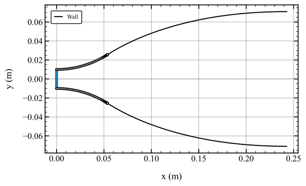
Nozzle wall contour mirrored about the centerline; both axes are in meters.

The wall opens downstream from the throat. The lower half is obtained by reflecting the computed upper wall about y = 0. Markers identify the initial initial front and points in the rounded expansion section.

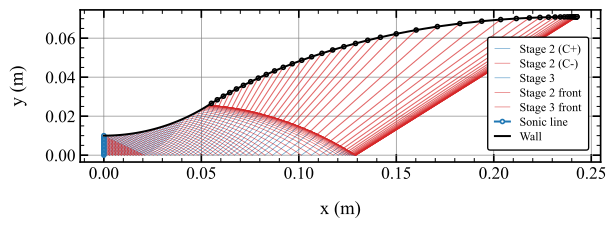
Characteristic mesh in the upper half of the nozzle.

The colored lines show the characteristic segments and marching fronts used to construct the solution. Their intersections carry the computed flow states. This view shows how the solution extends from the flat initial front into the expansion and downstream wall region.

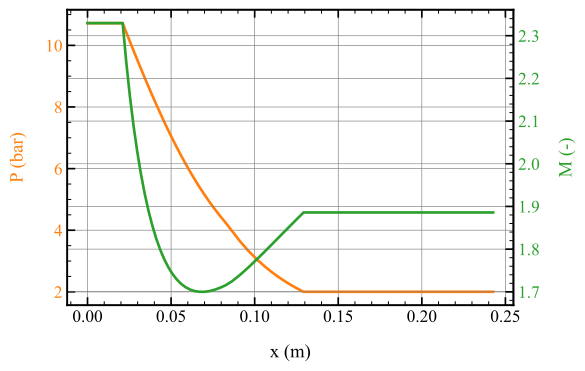
Pressure and Mach number along the nozzle centerline.

Read pressure against the left axis in bar and Mach number against the right axis. The pressure decrease accompanies supersonic acceleration, but Mach number can decrease locally as sound speed changes, as explained in the theory guide. The plotting helper extends the last centerline state to the exit with a constant segment.

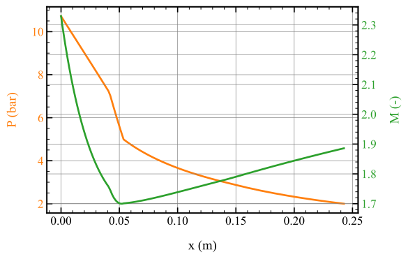
Pressure and Mach number along the computed nozzle wall.

This plot follows the wall instead of the centerline. Compare it with the previous plot to see how the expansion develops at different positions across the nozzle. Both use axial distance, rather than distance along the contour.

Use the exported results

The script prints the absolute path to examples/output/nozzle_design/. It saves four SVG figures and two CSV files:

File	Contents
wall_upper.csv	Computed upper wall from throat to exit.
wall_lower.csv	Mirrored lower wall in the same point order.

Both CSV headers are x_m,y_m; any upstream convergent section drawn by the plotter is outside these exported wall_final coordinates. Rerunning the script replaces the files in this directory.

Try changing Q0 to another value between zero and one or changing p_back, then compare the contour and property plots. Continue with the stator tutorial to turn the nozzle wall into a blade.