Build a stator blade from a two-phase nozzle

This example solves a cyclopentane expansion using the stator design conditions in Cioffi et al. [2026], then uses its wall to construct a stator blade profile. You will see how nozzle flow design and blade geometry fit together, and export both the source wall and the fitted blade.

Configure the nozzle and blade

The nozzle starts at 2.513 bar with a vapor mass fraction of 0.025 and expands toward a back pressure of 0.95 bar using the conventional solver and the curved Sauer initial line. Its throat half-height is 0.01 m. These are the paper’s operating conditions; the current package’s blade parametrization differs from the paper’s control-point construction, as discussed in stator theory.

Blade input	Value	Meaning
metal_angle_in	0.0 degrees	Camberline angle at the convergent-section inlet.
metal_angle_out	70.0 degrees	Camberline angle at the throat.
r_trailing	0.5 mm	Radius used to construct the trailing edge.
n_blades	2	Number of repeated profiles drawn by the plotter.
show_control_points	False	Hide the spline control polygon in the figure.

parametrize_stator_blade takes the nozzle wall in meters and constructs the blade in millimeters. It adds the convergent geometry and pressure side, then fits the blade contour with a B-spline. The plot repeats this geometry at the calculated pitch; n_blades changes only the display.

Run and inspect the script

Run from the repository root after following the source installation instructions:

poetry run python examples/moc_design/stator_design.py

The code below is included directly from the example. The final display block is omitted; the script opens the figures with plt.show() during normal runs.

from pathlib import Path

import matplotlib.pyplot as plt
import numpy as np

import turbo_moc
from turbo_moc.reporting import logging_context

from turbo_moc.geometry import parametrize_stator_blade

# 1. Cyclopentane stator design conditions from Cioffi et al. (2026),
#    Table 3. This uses the current package geometry, not an exact reproduction
#    of the paper's control-point construction.
# Show the solver's progress on the console (INFO; use level="DEBUG" for details).
with logging_context():
    data = turbo_moc.design_nozzle(
        fluid_name="Cyclopentane",
        P0=2.513e5,  # Stagnation pressure [Pa].
        Q0=0.025,  # Two-phase inlet: 2.5% vapor by mass.
        p_back=0.95e5,  # Design exit pressure [Pa].
        solver="conventional",
        use_true_sauer_line=True,  # Smooth sonic transition within the mixture.
    )

if not data["converged"] or not data["wall_final"]["x"]:
    raise RuntimeError("The nozzle design did not converge.")

wall = data["wall_final"]

# Nozzle coordinates are in meters; the stator geometry is returned in mm.
blade = parametrize_stator_blade(
    wall["x"],
    wall["y"],
    metal_angle_in=0.0,
    metal_angle_out=70.0,
    r_trailing=0.5,
    inlet_opening_ratio=1.5,
)

curve = blade["blade_curve"]
if not np.isfinite(np.column_stack((curve["x"], curve["y"]))).all():
    raise RuntimeError("The stator design produced invalid coordinates.")

# Plotting helpers return (figure, axes); keep the figures for SVG export.
figures = {
    "nozzle_contour": turbo_moc.mpl.plot_nozzle_contour(data)[0],
    "characteristics_mesh": turbo_moc.mpl.plot_characteristics_mesh(data)[0],
    "axis_properties": turbo_moc.mpl.plot_axis_properties(data)[0],
    "wall_properties": turbo_moc.mpl.plot_wall_properties(data)[0],
}
figures["stator_blade"] = turbo_moc.mpl.plot_blade(
    blade,
    n_blades=2,
    show_control_points=False,
)[0]

print(f"Stator pitch: {blade['pitch']:.4f} mm")
# Resolve output relative to this script, regardless of the working directory.
outdir = Path(__file__).resolve().parents[1] / "output" / "stator_design"
outdir.mkdir(parents=True, exist_ok=True)
np.savetxt(
    outdir / "nozzle_wall.csv",
    np.column_stack((wall["x"], wall["y"])),
    delimiter=",",
    header="x_m,y_m",
    comments="",
)
for name in ("blade_curve", "suction", "pressure", "trailing_edge"):
    surface = blade[name]
    np.savetxt(
        outdir / f"{name}.csv",
        np.column_stack((surface["x"], surface["y"])),
        delimiter=",",
        header="x_mm,y_mm",
        comments="",
    )
# Save vector figures that can also be embedded in the documentation.
for name, figure in figures.items():
    figure.savefig(outdir / f"{name}.svg", bbox_inches="tight")
print(f"Coordinates and figures saved to: {outdir}")

Read the figures

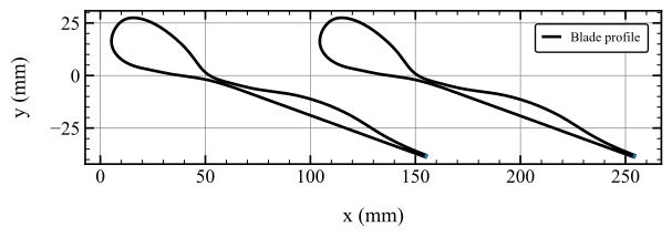
Two stator profiles repeated at the design pitch, with coordinates in millimeters.

The spacing between the two profiles forms the passage. The fitted contour and separate trailing-edge curve show the blade geometry assembled from the nozzle wall. The script prints the pitch of the resulting profile. Set show_control_points=True to see the points controlling the spline fit.

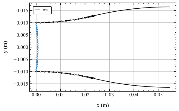
Source nozzle used to construct the stator, with coordinates in meters.

This is the flow-design input to the blade parametrization. Its wall provides the divergent-section suction-side geometry before the blade construction transforms and supplements it.

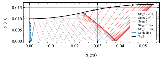
Characteristic solution for the source nozzle.

The mesh belongs to the nozzle calculation. The subsequent blade parametrization constructs geometry from that result; it does not compute a new flow solution through the complete stator passage.

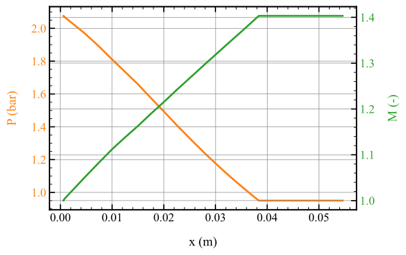
Centerline pressure and Mach number for the source nozzle.

Pressure uses the left axis in bar and Mach number uses the right axis. These curves describe the nozzle expansion that underlies the blade design.

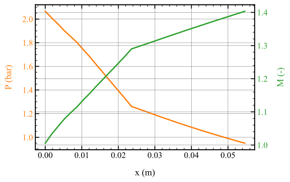
Wall pressure and Mach number for the source nozzle.

These are the flow states along the original nozzle wall. The horizontal coordinate is the nozzle axial position in meters, before the geometry is transformed into the stator profile.

Use the exported results

Results are written to examples/output/stator_design/, and the script prints the absolute path. Five SVG figures accompany these coordinate files:

File	Contents	Units
nozzle_wall.csv	Source nozzle wall, from throat to exit.	m
blade_curve.csv	Fitted B-spline contour.	mm
suction.csv	Constructed suction-side points.	mm
pressure.csv	Constructed pressure-side points.	mm
trailing_edge.csv	Separate trailing-edge curve.	mm

Keep the trailing-edge curve with the fitted contour when using the exported profile. CSV headers explicitly identify the units; the source nozzle wall must be scaled before combining it with blade coordinates.

Try changing metal_angle_out or r_trailing while leaving the nozzle inputs fixed. The blade geometry and pitch change, while the source nozzle solution stays the same.