Stator blade construction

The MoC produces a nozzle wall and its inviscid design flow. A stator profile requires additional geometry: a convergent inlet, a neighboring passage wall, finite leading and trailing edges, and periodic spacing. These operations embed the divergent contour into a blade cascade [Cioffi et al., 2026].

Passage and blade geometry

The two symmetric walls of a nozzle bound a flow passage. In a periodic cascade, the surfaces bounding that passage belong to adjacent blades. A solid blade is obtained by pairing a surface with the appropriate pitch-translated neighbor and closing the ends. Confusing the passage with the solid profile leads to incorrect blade thickness or spacing.

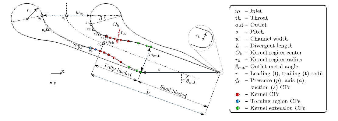
Stator construction extracted from Fig. 2 of Cioffi et al. [2026]. The source’s pitch \(s\) is \(t_b\) here, and its outlet metal angle \(\theta_\mathrm{out}\) is \(\chi\). The sketch explains the passage geometry; the current parametrization functions use the construction described below.

Review note — figure legend

The source figure’s legend and accompanying prose interchange the colors of the turning-region and kernel-extension control points. Use the geometric labels to interpret the sketch and reconcile the colors before preparing a replacement figure.

The fully bladed region is bounded by two blade surfaces. Beyond the shorter surface’s trailing edge, the passage becomes semi-bladed. These terms describe the flow domain; they are separate from the full and semi geometry variants implemented by the package.

Pitch, widths, and metal angle

For the mirrored-wall construction, let \(w_\mathrm{out}\) be the full nozzle opening normal to its exit direction. Adding the trailing-edge diameter and projecting the cascade pitch onto this normal gives

(1)\[t_b\cos\chi=w_\mathrm{out}+2r_\mathrm{TE},\qquad t_b=\frac{w_\mathrm{out}+2r_\mathrm{TE}}{\cos\chi}.\]

For a monotonically diverging symmetric nozzle, the implementation uses \(w_\mathrm{out}=2\max(y_w)\) after converting the MoC coordinates to millimeters. It sets the divergent axial chord to \((\max x_w-\min x_w)\cos\chi\) and the convergent axial chord to half that value. The inlet opening is determined by the input ratio inlet_opening_ratio, defined as pitch divided by inlet opening.

The semi variant uses a different passage construction and computes \(t_b=[\max(y_w)+2r_\mathrm{TE}]/\cos\chi\). The missing factor of two is part of that implementation; the symmetric-nozzle width interpretation cannot be transferred to it without checking the actual neighboring surfaces.

Review note — width conventions

Both stator functions return throat_opening from the first upper-wall ordinate. For a symmetric MoC nozzle this is the half-height, whereas the full nozzle throat width is \(2y_t\). Check terminology and the effective throat of the assembled and fitted passage, especially for the semi variant. The pitch formulas above describe the current code rather than an independent guarantee of its minimum passage opening.

Convergent portion and surface assembly

The current implementation constructs the convergent suction portion from a linearly varying metal angle. With \(\xi\) measured along its construction axis,

(2)\[\chi_c(\xi)=\chi_\mathrm{in} +(\chi_\mathrm{out}-\chi_\mathrm{in})\frac{\xi}{c_{a,\mathrm{conv}}}, \qquad \frac{\mathrm d\eta_c}{\mathrm d\xi}=\tan\chi_c(\xi).\]

The integrated curve is rotated and translated to join the MoC suction wall. Angles in this equation are radians; the API accepts degrees and converts them for trigonometric evaluation. This construction differs from the two cubic Bézier convergent curves described in the supplied paper.

For parametrize_stator_blade, the opposite divergent surface is obtained by reflection and pitch translation of the nozzle wall. A reflected prefix extends the throat neighborhood upstream. A cubic Hermite bridge connects the leading-edge region to this pressure surface. Its endpoint positions and tangent directions determine the shape, with tangent magnitudes setting how quickly the bridge turns.

For endpoint positions \(\boldsymbol P_0,\boldsymbol P_1\) and tangent vectors \(\boldsymbol d_0,\boldsymbol d_1\), the Hermite representation is

(3)\[\boldsymbol C(q)=(2q^3-3q^2+1)\boldsymbol P_0 +(q^3-2q^2+q)\boldsymbol d_0 +(-2q^3+3q^2)\boldsymbol P_1 +(q^3-q^2)\boldsymbol d_1,\qquad 0\leq q\leq1.\]

The parametrize_stator_blade_semi function instead constructs the pressure side from a circular arc between points near the two edges, followed by its connecting segments. It therefore changes more than the fitting procedure: the pressure-side geometry is no longer a mirrored MoC wall. Both variants add a leading-edge closure and a finite trailing-edge arc, then assemble a baseline profile.

B-spline representation

A cubic B-spline represents the sampled baseline with fewer control points:

(4)\[\boldsymbol C(q)=\sum_{j=0}^{n_c-1}N_{j,3}(q)\boldsymbol P_j.\]

The basis functions \(N_{j,3}\) are determined by the knot vector. The code first resamples the baseline approximately uniformly in arc length and then obtains the control points by least squares. The full variant fixes the endpoints of the fitted contour; the semi variant uses an unconstrained endpoint fit. The trailing-edge arc is also available separately in the output.

Position continuity requires adjoining curves to meet. Tangent continuity additionally requires their endpoint directions to agree; curvature continuity is a stronger condition. Neither a visually smooth plot nor a cubic degree alone guarantees that all joins preserve the intended throat and exit shape. The fit should be checked against the baseline and neighboring blade surfaces.

Review note — geometric fidelity

The paper reports a maximum contour deviation of 0.05 mm for its fitted geometry. The current functions accept a control-point count and sampling resolutions; they do not enforce that published maximum-deviation tolerance. Check the fitted throat width, end connections, and wall displacement before assigning a tolerance to the package output.

The stator example demonstrates the conversion from a cyclopentane nozzle into a blade profile. The resulting section can be used directly in a planar cascade or passed to the radial mapping functions. Its flow performance remains a subject for subsequent CFD analysis.