Design a two-phase vortex-flow rotor

Design a two-phase vortex-flow rotor#

This example constructs a supersonic rotor blade using the vortex-flow design function. You will specify a relative inlet state and Mach numbers, inspect the passage surfaces and assembled blade, and export dimensional coordinates.

The rotor is an independent design example. It does not read the stator output or match a complete turbine stage.

Configure the relative flow#

The inlet is a saturated nitrogen mixture at a relative stagnation pressure of 20 bar and vapor mass fraction of 0.5. The script obtains its saturation temperature through jaxprop, because the rotor API also requires a temperature argument.

Input	Value	Meaning
`M_inlet`	`1.6`	Relative Mach number upstream of the blade.
`M_outlet`	`1.2`	Relative Mach number downstream of the blade.
`M_lower`	`1.1`	Mach number on the pressure-side constant-Mach arc.
`M_upper`	`2.0`	Mach number on the suction-side constant-Mach arc.
`beta_inlet`	`5.0` degrees	Relative inlet flow angle from the axial direction.
`r_star`	`0.01` m	Sonic-streamline radius used to scale the geometry.
`num_points`	`60`	Number of points per transition arc.

The solver derives the outlet flow angle from mass-flux continuity. The wall-arc Mach numbers and the upstream/downstream Mach numbers control different parts of the construction. The inlet and outlet Mach numbers differ here, so the flow is not a constant-Mach impulse example.

Run and inspect the script#

Run from the repository root after following the source installation instructions:

poetry run python examples/moc_design/rotor_design.py

The code below is included directly from the example. The final display block is omitted; the script opens the figures with plt.show() during normal runs.

from pathlib import Path

import matplotlib.pyplot as plt
import numpy as np
import jaxprop as jxp

import turbo_moc

from turbo_moc.rotor import design_rotor_vortex_blade

# 1. Resolve the saturated inlet state in the rotor-relative frame.
pressure = 20e5
quality = 0.5
temperature = float(jxp.Fluid("nitrogen").get_state(jxp.PQ_INPUTS, pressure, quality).T)

# 2. Set the inlet/outlet Mach numbers and the two constant-Mach wall arcs.
# The solver derives the outlet angle; r_star sets the physical length scale.
data = design_rotor_vortex_blade(
    fluid_name="nitrogen",
    P0_rel=pressure,  # Relative stagnation pressure [Pa].
    T0_rel=temperature,  # Saturation temperature [K]; required by the rotor API.
    Q0_rel=quality,  # Relative stagnation vapor mass fraction.
    M_inlet=1.6,
    M_outlet=1.2,
    M_lower=1.1,
    M_upper=2.0,
    beta_inlet=5.0,
    r_star=0.01,  # Sonic-streamline radius [m]; gives dimensional coordinates.
    num_points=60,
)

blade = data["blade"]
if (
    not blade["x"]
    or not np.isfinite(data["solidity"])
    or not np.isfinite(np.column_stack((blade["x"], blade["y"]))).all()
):
    raise RuntimeError("The rotor design produced invalid blade geometry.")

# Plotting helpers return (figure, axes); keep the figures for SVG export.
figures = {
    "rotor_blade": turbo_moc.mpl.plot_rotor_vortex_blade(
        data,
        show_surfaces=False,
    )[0],
    "rotor_passage": turbo_moc.mpl.plot_rotor_blade(data)[0],
}
print(
    f"Pitch: {data['pitch']:.6f} m  Chord: {data['chord']:.6f} m  "
    f"Solidity: {data['solidity']:.4f}"
)

# Resolve output relative to this script, regardless of the working directory.
outdir = Path(__file__).resolve().parents[1] / "output" / "rotor_design"
outdir.mkdir(parents=True, exist_ok=True)
# Export the assembled blade; passage surfaces have their own local frames.
np.savetxt(
    outdir / "blade.csv",
    np.column_stack((blade["x"], blade["y"])),
    delimiter=",",
    header="x_m,y_m",
    comments="",
)
for name in ("pressure", "suction"):
    surface = data[name]
    np.savetxt(
        outdir / f"{name}_local.csv",
        np.column_stack((surface["x"], surface["y"])),
        delimiter=",",
        header="x_m,y_m",
        comments="",
    )
# Save vector figures that can also be embedded in the documentation.
for name, figure in figures.items():
    figure.savefig(outdir / f"{name}.svg", bbox_inches="tight")
print(f"Coordinates and figures saved to: {outdir}")

Read the figures#

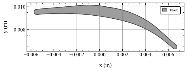
Assembled rotor blade with rounded leading and trailing edges, in meters.#

The filled region is the solid blade cross-section. The construction positions the two walls and joins them using straight segments and circular edge arcs. This is the geometry exported in blade.csv.

For these settings, the printed pitch is approximately 0.004753 m and the chord is 0.012298 m, giving a solidity of approximately 2.5875. Solidity is chord divided by pitch.

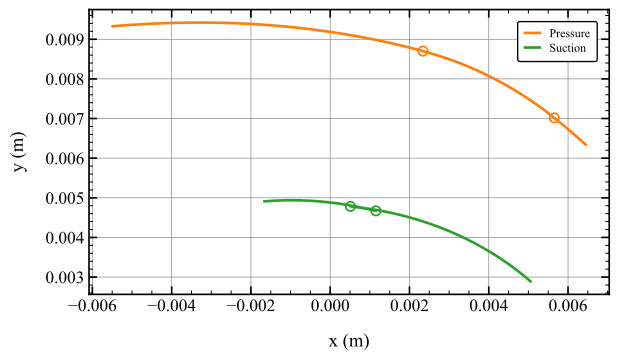
Pressure and suction passage surfaces with transition-arc junctions marked.#

This view shows the two flow-design surfaces before the blade closure. The hollow circles mark the junctions between the transition regions and constant-Mach circular arcs. The surfaces are exported in their own local frames; they should not be concatenated directly to form the solid blade shown above.

Use the exported results#

The script prints the absolute path to examples/output/rotor_design/. It saves two SVG figures and three coordinate files, all with x_m,y_m headers:

File	Contents
`blade.csv`	Assembled blade contour, including edge closure.
`pressure_local.csv`	Pressure-side surface in its local frame.
`suction_local.csv`	Suction-side surface in its local frame.

Use blade.csv when you need the complete profile. The local surface files are useful for examining the flow-design construction.

Try changing r_star to scale the blade. With the flow inputs unchanged, the lengths scale while solidity stays the same. Increasing num_points gives more points along each transition arc. Changing the Mach numbers or inlet angle changes the underlying flow design and derived outlet angle.