Coons patch

A Coons patch fills the region between four boundary curves. It blends the ruled surfaces between opposite boundaries and subtracts their shared bilinear corner contribution:

\[\begin{split}\begin{aligned} \mathbf S(u,v) &=(1-v)\mathbf C_{\rm south}(u)+v\mathbf C_{\rm north}(u)\\ &\quad +(1-u)\mathbf C_{\rm west}(v)+u\mathbf C_{\rm east}(v) -\mathbf B(u,v). \end{aligned}\end{split}\]

Here \(\mathbf B\) is the bilinear interpolant of the four corners. This expression describes the polynomial cubic Bézier example below.

Boundary orientation and compatibility

South and north run west to east. West and east run south to north. Their endpoints must agree:

Corner	Matching endpoints
Southwest	south(0) = west(0)
Southeast	south(1) = east(0)
Northwest	north(0) = west(1)
Northeast	north(1) = east(1)

nurbspy.nurbs_surface_coons.NurbsSurfaceCoons requires matching degrees, knot vectors, and control-point counts for opposite boundaries, as well as matching corner positions and weights. All four curves here are polynomial cubic Bézier curves with unit weights. This makes the class’s control-net blending agree with the classical Coons formula.

Complete script

Run python demos/documentation/coons_patch.py, or download the script.

"""Fill four compatible Bezier boundary curves with a Coons patch."""
import numpy as np
import matplotlib.pyplot as plt
import nurbspy as nrb

nrb.set_plot_options()

# South and north run west to east; west and east run south to north.
south = nrb.NurbsCurve(np.array([[0., 1., 2., 3.],
                                 [0., 0., 0., 0.],
                                 [0., -0.4, -0.4, 0.]]))
north = nrb.NurbsCurve(np.array([[0., 1., 2., 3.],
                                 [2., 2., 2., 2.],
                                 [0.5, 1.4, 1.4, 0.5]]))
west = nrb.NurbsCurve(np.array([[0., 0., 0., 0.],
                                [0., 2/3, 4/3, 2.],
                                [0., 0.8, 1.1, 0.5]]))
east = nrb.NurbsCurve(np.array([[3., 3., 3., 3.],
                                [0., 2/3, 4/3, 2.],
                                [0., -0.3, 0.2, 0.5]]))
surface = nrb.NurbsSurfaceCoons(
    C_south=south, C_north=north, C_west=west, C_east=east,
).NurbsSurface

t = np.linspace(0., 1., 61)
boundaries = [
    ("south", south, t, np.zeros_like(t)),
    ("north", north, t, np.ones_like(t)),
    ("west", west, np.zeros_like(t), t),
    ("east", east, np.ones_like(t), t),
]
print("Control net shape:", surface.P.shape)
print(f"Degrees: ({surface.p}, {surface.q})")
for name, curve, u, v in boundaries:
    error = np.max(np.abs(surface.get_value(u, v) - curve.get_value(t)))
    print(f"Maximum {name} boundary error: {error:.2e}")

fig, ax = surface.plot(surface_color=nrb.COLORS_MATLAB[0],
                       boundary=False, isocurves_u=9, isocurves_v=9)
for _, curve, _, _ in boundaries:
    curve.plot_curve(fig, ax, color=nrb.COLORS_MATLAB[1], linewidth=2.5)
ax.set_title("Coons patch bounded by four curves")
ax.view_init(elev=30, azim=-55)
# Leave room for the 3D axis labels when displaying or exporting the figure.
fig.set_size_inches(7, 6)
fig.subplots_adjust(left=0.05, right=0.85, bottom=0.15, top=0.9)
ax.set(xlabel="$x$", ylabel="$y$", zlabel="$z$")
for axis in (ax.xaxis, ax.yaxis, ax.zaxis):
    axis.labelpad = 4
plt.show()

Output

The resulting control net has shape (3, 4, 4) and degrees \((3,3)\). The script compares all four surface boundaries against the input curves, at 61 samples per boundary. The discrepancies are at floating-point roundoff.

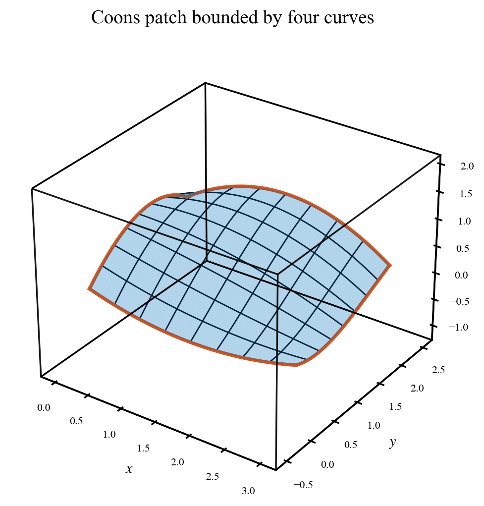
The patch interpolates all four orange boundary curves.

surface.plot() draws the patch and its parameter lines, while curve.plot_curve() highlights each boundary. Boundary interpolation specifies positions along the edges; matching tangent planes or curvature to adjacent surfaces requires additional constraints.