Ruled surface

A ruled surface connects corresponding points on two boundary curves by straight lines. For the polynomial curves in this example,

\[\mathbf S(u,v)=(1-v)\mathbf C_1(u)+v\mathbf C_2(u).\]

The \(u\) parameter follows each generating curve; increasing \(v\) moves along a straight ruling between them.

Inputs

nurbspy.nurbs_surface_ruled.NurbsSurfaceRuled takes two curves with matching control-point array shapes, degrees, and knot vectors. The example uses two quadratic Bézier curves with unit weights, so those requirements hold automatically. Its surface has degrees \((2,1)\).

For rational input curves with different weight functions, this helper blends their homogeneous representations. Each ruling remains straight, but v is generally a rational parametrization along it; the linear blend above applies when both weight functions agree, as they do here.

Complete script

Run python demos/documentation/ruled_surface.py, or download the script.

"""Connect two quadratic Bezier curves by straight rulings."""
import numpy as np
import matplotlib.pyplot as plt
import nurbspy as nrb

nrb.set_plot_options()

P1 = np.array([[0., 1.5, 3.],
               [0., 0., 0.],
               [0., 1.5, 0.]])
P2 = np.array([[0., 1.5, 3.],
               [2., 2., 2.],
               [1., 0.2, 1.5]])
C1 = nrb.NurbsCurve(control_points=P1)
C2 = nrb.NurbsCurve(control_points=P2)
surface = nrb.NurbsSurfaceRuled(C1, C2).NurbsSurface

u = np.linspace(0., 1., 61)
v = np.full_like(u, 0.35)
expected = (1 - v) * C1.get_value(u) + v * C2.get_value(u)
error = np.max(np.abs(surface.get_value(u, v) - expected))
print("Control net shape:", surface.P.shape)
print(f"Degrees: ({surface.p}, {surface.q})")
print(f"Maximum linear-blend error: {error:.2e}")
print("Midpoint:", surface.get_value(0.5, 0.5)[:, 0].round(6))

fig, ax = surface.plot(surface_color=nrb.COLORS_MATLAB[0],
                       isocurves_u=13, isocurves_v=3)
C1.plot_curve(fig, ax, color=nrb.COLORS_MATLAB[1], linewidth=2.5)
C2.plot_curve(fig, ax, color=nrb.COLORS_MATLAB[1], linewidth=2.5)
ax.set_title("Ruled surface between two curves")
ax.view_init(elev=25, azim=-55)
# Leave room for the 3D axis labels when displaying or exporting the figure.
fig.set_size_inches(7, 6)
fig.subplots_adjust(left=0.05, right=0.85, bottom=0.15, top=0.9)
ax.set(xlabel="$x$", ylabel="$y$", zlabel="$z$")
for axis in (ax.xaxis, ax.yaxis, ax.zaxis):
    axis.labelpad = 4
plt.show()

Output

The control net has shape (3, 3, 2). The midpoint is [1.5    1.     0.7375]. The script checks the linear-blend formula at 61 values of \(u\) with \(v=0.35\); the error is at floating-point roundoff.

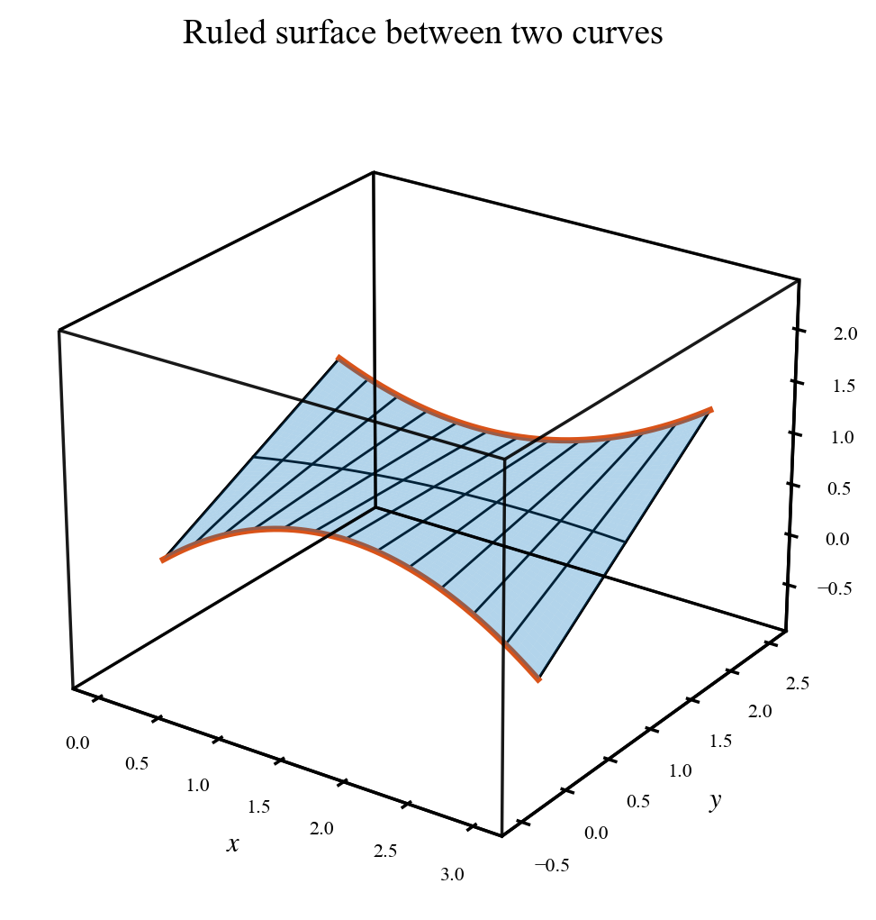
The orange curves generate the patch; the straight black lines hold \(u\) fixed.

surface.plot() draws the patch and its isoparametric curves. Each boundary’s plot_curve() method highlights the generating geometry.