Surface of revolution: a torus

A torus is formed by revolving an offset circle about an axis in its plane. Here the generating circle has radius \(r=0.6\), its center is at \((R,0,0)\) with \(R=2\), and the axis is the \(z\) axis. A full \(2\pi\) rotation creates a ring torus, since \(R>r\).

Inputs and parameters

First create the exact circular profile with CircularArc. Then pass its .NurbsCurve to nurbspy.nurbs_surface_revolution.NurbsSurfaceRevolution, together with the axis point, axis direction, and angular limits. The constructor keywords are angle_start and angle_end, in radians.

For this surface, \(u\) follows the revolution and \(v\) follows the profile. Both parameters are normalized to \([0,1]\); they are not the angles themselves. The familiar angular parametrization explains the geometry:

\[\begin{split}\begin{aligned} x&=(R+r\cos\phi)\cos\theta,\\ y&=(R+r\cos\phi)\sin\theta,\\ z&=r\sin\phi. \end{aligned}\end{split}\]

Its parameter-independent identity is

\[\left(\sqrt{x^2+y^2}-R\right)^2+z^2=r^2.\]

Complete script

Run python demos/documentation/revolution_surface.py, or download the script.

"""Revolve a circular profile about the z axis to make an exact torus."""
import numpy as np
import matplotlib.pyplot as plt
import nurbspy as nrb

nrb.set_plot_options()

major_radius, minor_radius = 2., 0.6
# The generating circle lies in the xz plane, offset from the z axis.
profile = nrb.CircularArc(
    O=np.array([major_radius, 0., 0.]),
    X=np.array([1., 0., 0.]),
    Y=np.array([0., 0., 1.]),
    R=minor_radius, theta_start=0., theta_end=2 * np.pi,
).NurbsCurve
surface = nrb.NurbsSurfaceRevolution(
    generatrix=profile,
    axis_point=np.array([0., 0., 0.]),
    axis_direction=np.array([0., 0., 1.]),
    angle_start=0., angle_end=2 * np.pi,
).NurbsSurface

# Here u follows the revolution; v follows the generating circle.
uu, vv = np.meshgrid(np.linspace(0., 1., 61), np.linspace(0., 1., 41),
                     indexing="ij")
S = surface.get_value(uu.ravel(), vv.ravel())
tube_radius = np.sqrt((np.hypot(S[0], S[1]) - major_radius)**2 + S[2]**2)
t = np.linspace(0., 1., 61)
u_seam = surface.get_value(np.zeros_like(t), t) - surface.get_value(np.ones_like(t), t)
v_seam = surface.get_value(t, np.zeros_like(t)) - surface.get_value(t, np.ones_like(t))
print("Control net shape:", surface.P.shape)
print(f"Degrees: ({surface.p}, {surface.q})")
print(f"Maximum tube-radius error: {np.max(np.abs(tube_radius - minor_radius)):.2e}")
print(f"Maximum u-seam mismatch: {np.max(np.abs(u_seam)):.2e}")
print(f"Maximum v-seam mismatch: {np.max(np.abs(v_seam)):.2e}")

fig, ax = surface.plot(surface_color=nrb.COLORS_MATLAB[0],
                       boundary=False, isocurves_u=17, isocurves_v=9,
                       Nu=121, Nv=81)
profile.plot_curve(fig, ax, color=nrb.COLORS_MATLAB[1], linewidth=2.5)
ax.set_title("Torus by revolution of a circle")
ax.view_init(elev=30, azim=-55)
# Leave room for the 3D axis labels when displaying or exporting the figure.
fig.set_size_inches(7, 6)
fig.subplots_adjust(left=0.05, right=0.85, bottom=0.15, top=0.9)
ax.set(xlabel="$x$", ylabel="$y$", zlabel="$z$")
for axis in (ax.xaxis, ax.yaxis, ax.zaxis):
    axis.labelpad = 4
plt.show()

Output

The control net has shape (3, 9, 9) and degrees \((2,2)\). Four rational quadratic spans close each circular direction. The script verifies the tube radius \(r\) and the coincidence of both pairs of parameter boundaries, with errors near machine precision.

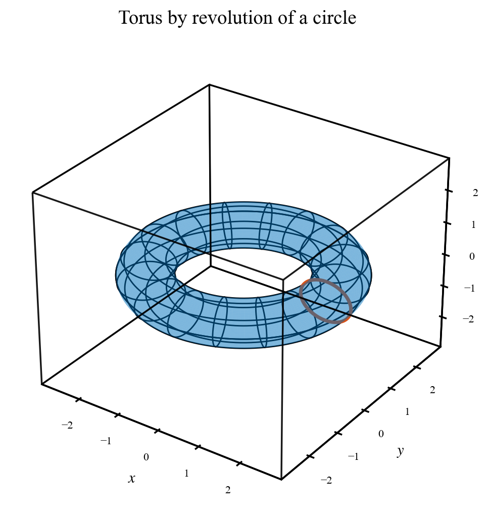
Revolving the orange circle produces the torus; black lines show the two parameter directions.

The plot uses surface.plot() and profile.plot_curve(). Reducing the revolution angle creates an open portion of the torus; other generating curves produce other surfaces of revolution.