Point projection onto a surface

The point-inversion problem

Point projection onto a surface \(\mathbf S(u,v)\) extends the curve problem to two parameters: given an external point \(\mathbf P\), find

\[(u^*, v^*) = \operatorname*{argmin}_{(u,v)\,\in\,[0,1]^2} \left\lVert \mathbf S(u,v) - \mathbf P \right\rVert.\]

At an interior minimum, the vector between \(\mathbf P\) and its closest point is orthogonal to both tangent directions of the surface there:

(1)\[\big(\mathbf S(u^*,v^*) - \mathbf P\big)\cdot \mathbf S_u(u^*,v^*) = 0, \qquad \big(\mathbf S(u^*,v^*) - \mathbf P\big)\cdot \mathbf S_v(u^*,v^*) = 0.\]

If the closest point lies on an edge or a corner of the patch instead, one or both of these conditions need not hold: the corresponding parameter is pinned at \(0\) or \(1\) by the domain boundary rather than by the surface bending away from \(\mathbf P\).

How nurbspy solves it

surface.project_point_to_surface(P) minimizes \(\lVert\mathbf S(u,v)-\mathbf P\rVert\) with SciPy’s L-BFGS-B, using the analytic gradient of that objective — the two orthogonality residuals in (1), normalized by the distance. As for curves, it evaluates every combination of knot-span midpoints in \(u\) and \(v\) first and starts the local optimization from whichever gives the smallest distance, which reduces but does not eliminate the risk of converging to the wrong local minimum on patches with several comparably close regions.

maxiter, ftol, and gtol control the underlying L-BFGS-B solve and default to 200, 1e-6, and 1e-6 respectively; pass tighter tolerances or a larger maxiter for hard-to-converge projections, or looser ones when only an approximate foot point is needed.

Script

Run python demos/documentation/point_projection_surface.py, or download the script.

"""Project external points onto a NURBS surface by minimizing distance to it."""
import numpy as np
import matplotlib.pyplot as plt
import nurbspy as nrb

nrb.set_plot_options()

x, y = np.meshgrid(np.linspace(0., 3., 4), np.linspace(0., 2., 3), indexing="ij")
z = np.array([[0., 1., 0.],
              [1., 2., 1.],
              [1., 2., 1.],
              [0., 1., 0.]])
P = np.stack([x, y, z])  # Shape (3, 4, 3): coordinates, u index, v index.
surface = nrb.NurbsSurface(control_points=P)

targets = np.array([[1.5, 3.5, 0.2],
                     [1.0, 0.5, 1.8],
                     [3.0, -0.5, 0.5]])

fig = plt.figure(figsize=(7, 6))
ax = fig.add_subplot(projection="3d")
surface.plot_surface(fig, ax, color=nrb.COLORS_MATLAB[0], alpha=0.5)

for i in range(targets.shape[1]):
    target = targets[:, i]
    # maxiter, ftol, and gtol are optional overrides for the underlying
    # L-BFGS-B solve; shown here at their defaults.
    u, v = surface.project_point_to_surface(target, maxiter=200, ftol=1e-6, gtol=1e-6)
    foot = surface.get_value(u, v)[:, 0]
    du = surface.get_derivative(u, v, order_u=1, order_v=0)[:, 0]
    dv = surface.get_derivative(u, v, order_u=0, order_v=1)[:, 0]
    orthogonality = (np.dot(foot - target, du), np.dot(foot - target, dv))
    print(f"Target {target}: (u,v)=({u:.6f}, {v:.6f}), foot={foot.round(6)}, "
          f"(S-P)*S_u,(S-P)*S_v={orthogonality[0]:.2e}, {orthogonality[1]:.2e}")
    ax.plot([target[0], foot[0]], [target[1], foot[1]], [target[2], foot[2]],
            "k--", marker="o", markerfacecolor="w", linewidth=1)

ax.set(xlabel="x", ylabel="y", zlabel="z", title="Point projection onto a NURBS surface")
plt.show()

Output

Target	\((u^*, v^*)\)	Foot point	Orthogonality
\((1.5,\ 1.0,\ 3.0)\)	\((0.500,\ 0.500)\)	\((1.5,\ 1.0,\ 1.25)\)	\((0,\ 0)\)
\((3.5,\ 0.5,\ -0.5)\)	\((1.000,\ 0.000)\)	\((3.0,\ 0.0,\ 0.0)\)	\((-3.0,\ 0)\)
\((0.2,\ 1.8,\ 0.5)\)	\((0.083,\ 0.878)\)	\((0.248,\ 1.756,\ 0.442)\)	\((6.3\times10^{-6},\ 2.2\times10^{-6})\)

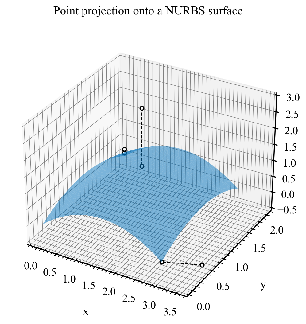
Two projections land on the boundary curves of the patch; the third lands in its interior.

The first target projects onto the interior, where both orthogonality residuals are at solver tolerance. The second is closest to the surface’s \(u=1\) boundary curve, so only the \(v\)-condition holds: \(v^*=0\) is pinned by the domain edge, and the nonzero \(u\)-residual reflects that. The third again lands in the interior.