Curve arc length and numerical integration

Arc length measures distance along a curve. It is used to compare designs, space points by distance, scale local reference frames and define geometric objectives such as bending energy. It is independent of how quickly the curve parameter moves through space.

The analytic derivatives used here are developed on the NURBS page. The geometry may be planar or spatial. Assume real control points, positive weights and a continuous curve over the integration interval.

From parameter increments to distance

For a curve \(\mathbf C(u)\), a small parameter increment gives \(d\mathbf C\approx\mathbf C'(u)\,du\). Its physical distance is

\[ ds=v(u)\,du,\qquad v(u)=\|\mathbf C'(u)\|, \qquad L(a,b)=\int_a^b v(u)\,du\quad(a\le b). \]

\(v\) is the parameter speed. It is not a physical velocity unless \(u\) is time. If coordinates have units of length and \(u\) is dimensionless, \(v\) also has units of length. Uniform increments in \(u\) generally do not give uniform increments in \(s\).

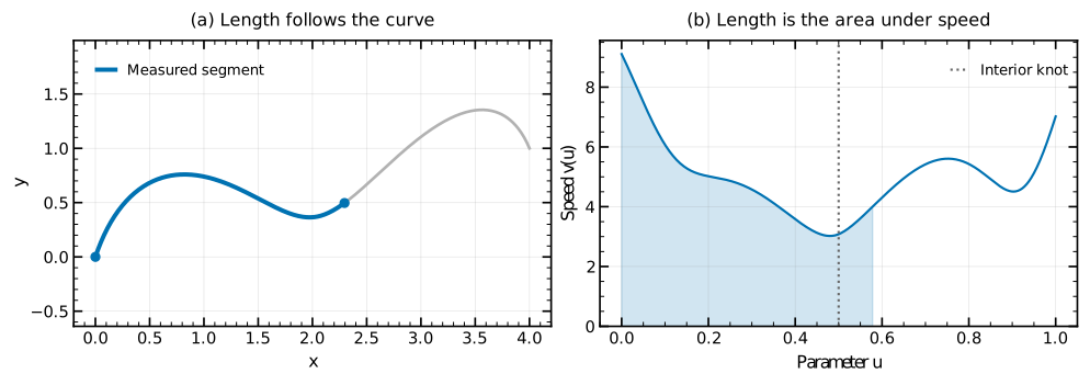
The highlighted segment and shaded speed integral describe the same length. The interior knot is marked in parameter space. Both plots are evaluated from the same rational cubic using get_value() and get_derivative().

The chord length \(\|\mathbf C(b)-\mathbf C(a)\|\) is a lower bound on arc length. A polyline through increasingly dense samples is useful as a diagnostic, but it also underestimates a curved segment and can miss a sharp feature.

Split the integral at knots

A NURBS curve is smooth within each nonzero knot span. Its derivatives can change at a knot, depending on degree and multiplicity. With clipped span boundaries \(a=t_0<\cdots<t_m=b\),

\[ L(a,b)=\sum_{k=0}^{m-1}\int_{t_k}^{t_{k+1}}v(u)\,du. \]

This keeps an integration panel from straddling a known change in smoothness. Repeated knots create zero-width spans, which contribute no length. A corner can have a perfectly valid length even though its tangent is discontinuous. A curve with a positional jump needs an explicit policy for the gap; the JAX adaptive and ODE APIs conservatively reject interior multiplicity above the degree rather than adding straight segments implicitly.

Three calculation approaches

Fixed quadrature

An integration rule replaces an integral by a weighted sum:

\[ \int_a^b v(u)\,du\approx \sum_{j=1}^{N}\omega_jv(u_j). \]

The nodes and weights include the mapping from the reference interval to \([a,b]\). Gauss–Legendre nodes are interior points; Clenshaw–Curtis nodes are distributed using cosine spacing and include the endpoints.

Fixed rules have predictable work and compact differentiable computations. They do not adapt if an important feature lies between the nodes. Even when \(\mathbf C\) is polynomial, its speed contains a square root and is not usually a polynomial integrated exactly by the rule.

JAX get_arclength_quad_fixed() uses one global Clenshaw–Curtis rule, with 41 nodes by default. The requested minimum node count rounds upward to a supported \(4k+1\) rule, with at least five nodes. Optional prepare_arclength() instead places Gauss–Legendre nodes within knot spans and stores the polynomial basis derivatives at those nodes. Changing control points and weights then requires only geometry evaluation and the weighted sum.

Adaptive quadrature

Adaptive Gauss–Kronrod quadrature compares two related rules to estimate local error. Panels with large estimated error are subdivided. The JAX default uses knot-aware Gauss–Kronrod integration and requests the combined target

\[ \text{estimated error}\le \max\!\left(\mathrm{atol},\,\mathrm{rtol}|L|\right). \]

The absolute tolerance has length units; the relative tolerance is dimensionless. The estimate is useful evidence, not a rigorous bound: both rules can miss an unsampled narrow layer. Large positive weight ratios trigger endpoint grading in the implementation to improve coverage of rational layers. Normalization and reflection improve floating-point resolution near endpoints; they cannot guarantee resolution of arbitrary interior features.

Integrating a length ODE

The same integral can be written as an initial-value problem:

\[ \frac{ds}{du}=v(u),\qquad s(a)=0,\qquad L(a,b)=s(b). \]

get_arclength_ode() uses an adaptive Runge–Kutta solver with knot boundaries explicitly respected. It is a useful alternative, particularly when reasoning about cumulative distance. Its tolerances control local ODE errors; they do not establish the same global error estimate as adaptive quadrature.

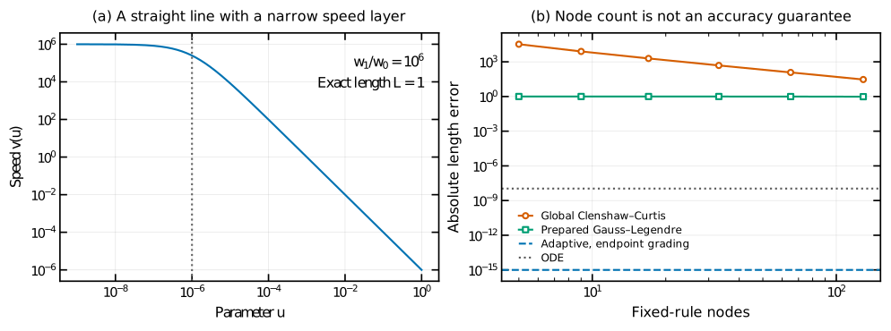
A straight rational line with weights \((1,10^6)\) has exact length one, yet its speed is concentrated near \(u=0\). The plotted estimates call the production JAX APIs. Increasing fixed-rule order alone can remain ineffective; the prepared rule here has one panel and no subdivisions. This is an accuracy example, not a timing comparison or a ranking for all geometries.

Choosing and calling a method

import jax.numpy as jnp
import nurbspy.jax as nrb

curve = nrb.NurbsCurve(jnp.array([[0., 0.5, 1.], [0., 1., 0.]]))
length = curve.get_arclength(atol=1e-10, rtol=1e-9)
partial = curve.get_arclength(0.2, 0.8, tol=1e-9)
fixed = curve.get_arclength_quad_fixed(n_points=65)
ode = curve.get_arclength_ode(tol=1e-9)
info = curve.get_arclength(return_info=True)

Situation	Starting choice
General length calculation with accuracy controls	get_arclength(), the adaptive default
Explicit adaptive entry point	get_arclength_quad_adaptive()
Alternative length integration	get_arclength_ode()
Small, validated fixed calculation	get_arclength_quad_fixed()
Repeated evaluations with changing control points/weights	prepare_arclength(), validated over the design family

The JAX dispatcher accepts static method="quad_adaptive", "quad_fixed" or "ode". tol supplies unspecified absolute and relative tolerances for adaptive/ODE integration; their effective default is \(10^{-6}\). Fixed quadrature accepts n_points and rejects tolerances. The old ambiguous get_arclength_quad() name is no longer provided.

For prepared evaluation:

table = nrb.prepare_arclength(curve, order=16, subdivisions=2)
length = table.value(curve.P, curve.W)

Rebuild when knots, degree, limits or quadrature resolution change. Supply weights explicitly for rational geometry: omitted weights mean unit weights. Validate prepared results against adaptive integration over the intended design family; agreement between two fixed orders can miss a shared blind spot.

The default NumPy backend has a different contract: nurbspy.NurbsCurve.get_arclength(a,b) uses a global 10-node Gauss–Legendre rule and does not expose these JAX method/tolerance options.

Sensitivities and numerical checks

For a design variable \(\theta\), where the speed is nonzero and differentiation under the integral is valid, the length derivative is

\[ \frac{dL}{d\theta}= v(b)\frac{db}{d\theta}-v(a)\frac{da}{d\theta} +\int_a^b \frac{\mathbf C'(u)\cdot\partial_\theta\mathbf C'(u)}{\|\mathbf C'(u)\|}\,du. \]

JAX adaptive integration offers adjoint="direct", which differentiates the accepted discretization, and adjoint="leibniz", which gives the derivative integration its own adaptive solve. A small primal error estimate does not certify a gradient. Check important sensitivities by tightening controls and comparing a directional derivative with an independent finite difference.

Scalar adaptive/ODE calls raise on failure. With return_info=True, inspect the returned value, status, work and error diagnostics instead: status zero means successful termination. ODE error estimates are unavailable and reported as NaN. Reversed limits return a signed integral; equal limits return zero. Use ordered limits when a positive physical length is intended.

Isolated zero speed does not necessarily invalidate length. The implementation selects a zero norm subgradient at exactly zero velocity, but this does not make the length of a completely collapsed curve differentiable. Inverting length is a separate problem with stronger regularity requirements, described on the parameterization page.

Reproduce the figures

python docs/generate_theory_images.py --only arclength

The figure script constructs the geometry, calls the public APIs and checks the exact rational-line length. Vector PDFs: curve and speed, integration comparison.