Surface differential geometry

Surface differential geometry turns partial derivatives into physical directions, lengths and bending measures. The main quantities are the tangent plane, oriented normal, local metric and curvatures. This page explains the calculations behind get_normals() and get_curvature() for a regular 3D surface \(\mathbf S(u,v)\).

Tangent plane and oriented normal

The two partial derivatives describe how position changes along the parameter directions:

\[ d\mathbf S=\mathbf S_u\,du+\mathbf S_v\,dv,\qquad \mathbf n=\frac{\mathbf S_u\times\mathbf S_v} {\|\mathbf S_u\times\mathbf S_v\|}. \]

\(\mathbf S_u\) and \(\mathbf S_v\) span the tangent plane when they are linearly independent. They need not be perpendicular or have unit length. Their cross product sets the normal’s orientation. Reversing one parameter direction reverses the normal; reversing both preserves it. The package does not infer an application-specific notion of outward direction from a collection of patches.

The first fundamental form: local distance

Taking the squared norm of \(d\mathbf S\) gives

\[ ds^2=E\,du^2+2F\,du\,dv+G\,dv^2, \qquad E=\mathbf S_u\cdot\mathbf S_u,\quad F=\mathbf S_u\cdot\mathbf S_v,\quad G=\mathbf S_v\cdot\mathbf S_v. \]

The matrix \(\mathrm I=\begin{pmatrix}E&F\\F&G\end{pmatrix}\) is the metric, or first fundamental form. It converts parameter increments to physical lengths. \(F=0\) means the two parameter directions are locally orthogonal. Regularity requires \(EG-F^2>0\), and the area scale factor is \(J_A=\sqrt{EG-F^2}\). See surface integration.

This explains why a unit step in \(u\) and a unit step in \(v\) are not generally comparable physical motions. The metric is also useful when diagnosing a stretched or nearly collapsed parameterization.

The second fundamental form: local bending

Project the second partial derivatives onto the normal:

\[\begin{split} e=\mathbf n\cdot\mathbf S_{uu},\qquad f=\mathbf n\cdot\mathbf S_{uv},\qquad g=\mathbf n\cdot\mathbf S_{vv},\qquad \mathrm{II}=\begin{pmatrix}e&f\\f&g\end{pmatrix}. \end{split}\]

These coefficients describe the surface’s bending away from the tangent plane. For a nonzero parameter direction \((\alpha,\beta)\), the signed normal curvature in that direction is

\[ k_n(\alpha,\beta)= \frac{e\alpha^2+2f\alpha\beta+g\beta^2} {E\alpha^2+2F\alpha\beta+G\beta^2}. \]

The denominator measures physical tangent length; the numerator measures bending toward the chosen normal. This ratio, rather than a raw second partial derivative, gives a geometrically meaningful curvature.

Principal, mean and Gaussian curvature

The extreme values of \(k_n\) are the principal curvatures \(k_1,k_2\). Their parameter directions solve \(\mathrm{II}\,\mathbf a=k\,\mathrm I\,\mathbf a\). Map a parameter direction \((\alpha,\beta)\) into the physical tangent vector \(\alpha\mathbf S_u+\beta\mathbf S_v\) before interpreting or plotting it.

The package returns mean curvature \(H\) and Gaussian curvature \(K\):

\[ H=\frac{k_1+k_2}{2} =\frac{Eg-2Ff+Ge}{2(EG-F^2)},\qquad K=k_1k_2=\frac{eg-f^2}{EG-F^2}. \]

\(H\) has inverse-length units; \(K\) has inverse-length-squared units. Reversing the normal changes the signs of \(e,f,g,k_1,k_2,H\), while \(K\) stays unchanged. With these definitions, a sphere with outward normal has \(H=-1/R\) and \(K=1/R^2\). A cylinder has \(K=0\) even though it bends in one direction.

Gaussian curvature	Local interpretation
\(K>0\)	Both principal curvatures have the same sign; locally dome-like
\(K<0\)	Principal curvatures have opposite signs; locally saddle-like
\(K=0\)	At least one principal curvature vanishes

From returned \(H,K\), principal curvature values can be recovered as \(k_{1,2}=H\pm\sqrt{H^2-K}\). Near an umbilic point, where the curvatures coincide, the principal directions are not uniquely determined. Roundoff can make \(H^2-K\) slightly negative; a tiny negative value may be clipped for display, but a substantial negative value signals a numerical or implementation problem. The package has no dedicated principal-direction or metric API; these are derived calculations using its partial derivatives.

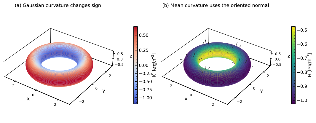
An exact rational torus with major radius 2 and tube radius 0.6. Gaussian curvature is positive on the outer side and negative on the inner side. Mean curvature uses the outward normals shown in the right panel, and is negative under the stated convention. Colors are computed from nurbspy’s analytic derivatives; no qualitative curvature field is imposed.

Calculate the quantities

Both backends expose the same surface geometry methods:

# surface is a regular 3D NurbsSurface; u and v are paired arrays.
su = surface.get_derivative(u, v, 1, 0)
sv = surface.get_derivative(u, v, 0, 1)
normal = surface.get_normals(u, v)       # Shape (3, N).
H, K = surface.get_curvature(u, v)       # Each shape (N,).

Use np.sum(su*sv, axis=0) for metric contractions with NumPy, or the JAX equivalent. Mixed derivative order (1,1) means \(\mathbf S_{uv}\); (2,0) and (0,2) mean \(\mathbf S_{uu}\) and \(\mathbf S_{vv}\). Values and partials pair the entries of \(u\) and \(v\); form a mesh explicitly for a grid.

For repeated changing-design calculations at fixed locations, JAX prepare_surface() can retain the basis tables. Prepare derivatives through order two for curvature and order one for normals or area. Changing the sampling layout or defining knots requires rebuilding those tables.

Degeneracy, knots and numerical sensitivity

At \(\mathbf S_u\times\mathbf S_v=0\), the normal and ordinary curvature formulas are undefined. This may describe a collapsed patch or a singular parameterization of an otherwise smooth physical surface, such as a pole. Do not interpret NaNs or very large curvature near such a point as reliable physical bending.

Curvature requires the relevant second derivatives. Repeated knots can reduce smoothness; distinguish one-sided curvature from a unique curvature at a join. Very different parameter scales and nearly parallel tangent directions can also make the metric poorly conditioned. Compare against analytic shapes and inspect the area Jacobian when results look suspicious.

Reproduce the figure

python docs/generate_theory_images.py --only surface_geometry

The figure script checks both curvatures against the analytic torus formulas and verifies unit normals. Download the vector PDF.